3D Geometry Compression

Java 3D API Specification

JAVA 3D allows programmers to specify geometry using a binary geometry compression format. This compression format is used with APIs other than just Java 3D, and can be used both as a runtime in-memory format for describing geometry, as well as a storage and network format. Eventually the full specification of the geometry compression format described in this section will be part of its own stand-alone specification, but for completeness it is included as an appendix to the early specification of the Java 3D API.
Java 3D uses a geometry compression format that allows 3D geometry to be represented in an order of magnitude less space than most traditional 3D representations, with very little loss in object quality. The compression is achieved through several layers of techniques.
This appendix attempts to completely specify all the details of the geometry compression format. To ensure current and future compatibility, it is essential to only use the features explicitly specified in this document. Any features, fields, usage, etc. not specified in the document should be considered "illegal". "Illegal" means that using such a construct will be incompatible with current implementations or will break future implementations. If something is illegal, don't use it. This document will point out many of the illegal constructs, but not all of them.

B.1 Compression
First, the geometry to be compressed is converted into a generalized mesh form, which allows a triangle to be, on average, specified by 0.80 vertices.
Next the data for each vertex component of the geometry is converted to the most efficient representation format for its type and then quantized to as few bits as possible.
These quantized bits are differenced between successive vertices, and the results are modified Huffman encoded into self-describing variable-bit-length data elements.
Finally, these variable-length elements are strung together using Java 3D's eight geometry commands into a final compressed geometry block.

B.2 Decompression
Upon receipt, compressed geometry blocks are decompressed into the local host's preferred geometry format by reversing the above process.

B.3 Appendix Organization
Before the bit details of the compression can be specified, several of the concepts used in geometry compression need elaboration. The first several sections are an expansion of our SIGGRAPH '95 paper on geometry compression.¹

Generalized Triangle Strip. This section is a refresher on the concept and semantics of a generalized triangle strip.

Generalized Triangle Mesh. This section introduces the concept and semantics of a generalized triangle mesh.

Position Representation and Quantization. This section describes the fixed-point format used for 3D positional representation.

Color Representation and Quantization. This section describes the fixed-point format used for color representation.

Normal Representation and Quantization. This section describes a novel folded table based representation of surface normals, and the fixed-point format of the resultant normals.

Modified Huffman Encoding. This section describes the variant of Huffman delta encoding used for geometry compression.

Geometry Compression Commands. This section gives an overview of the eight geometry compression commands.

B.4 Generalized Triangle Strip
A generalized triangle strip is a generalization of the concept of a "zig-zag" and "star" triangle strip. It is a sequence of vertices in which each vertex contains a two-bit replacement code. This replacement code defines how the present vertex is to be combined with previous vertices to form the next triangle. The replacement bits can also be thought of as a generalization of the "move/draw" bit used for lines.
A stack of the last three vertices used to form a triangle is kept. The three vertices are labeled oldest, middle, and newest. An incoming vertex of type replace_oldest causes the oldest vertex to be replaced by the middle, the middle to be replaced by the newest, and the incoming vertex to become the newest. This corresponds to a PHIGS PLUS triangle strip (sometimes called a "zig-zag" strip). The replacement type replace_middle leaves the oldest vertex unchanged, replaces the middle vertex by the newest, and the incoming vertex becomes the newest. This corresponds to a triangle star or fan.
The replacement type restart marks the oldest and middle vertices as invalid, and the incoming vertex becomes the newest. Generalized triangle strips must always start with this code. A triangle will be output only when a replacement operation results in three valid vertices.
Restart corresponds to a "move" operation in polylines, and allows multiple unconnected variable-length triangle strips to be described by a single data structure passed in by the user, reducing the overhead. The generalized triangle strip's ability to effectively change from "strip" to "star" mode in the middle of a strip allows more complex geometry to be represented compactly, and requires less input data bandwidth. The restart capability allows several pieces of disconnected geometry to be passed as one data block. Figure B-1 shows a single generalized triangle strip and the associated replacement codes.
Triangles are normalized such that the front face is always defined by a clockwise vertex order after transformation. To support this, there are two flavors of restart: restart_clockwise and restart_counterclockwise. The vertex order is reversed after every replace_oldest, but remains the same after every replace_middle.

B.5 Generalized Triangle Mesh
The first stage of geometry compression is to convert triangle data into an efficient linear strip form: the generalized triangle mesh. This is a near-optimal representation of triangle data, given fixed storage.
The existing concept of a generalized triangle strip structure allows for compact representation of geometry while maintaining a linear data structure. That is, the geometry can be extracted by a single monotonic scan over the vertex array data structure. This is very important for pipelined hardware implementations, a data format that requires random access back to main memory during processing is very problematic.

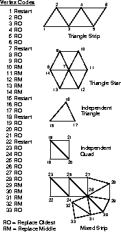
Figure B-1 A Generalized Triangle Strip

However, by confining itself to linear strips, the generalized triangle strip format leaves a potential factor of two (in space) on the table. Consider the geometry in Figure B-2.
While it can be represented by one triangle strip, many of the interior vertices appear twice in the strip. This is inherent in any approach wishing to avoid references to old data. Some systems have tried using a simple regular mesh buffer to support reuse of old vertices, but there is a problem with this approach in practice: In general, geometry does not come in a perfectly regular rectangular mesh structure.

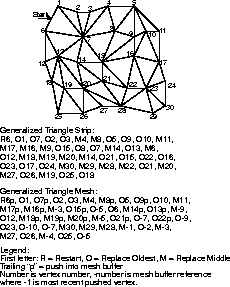
Figure B-2 A Generalized Triangle Mesh

The generalized technique employed by geometry compression addresses this problem. Old vertices are explicitly pushed into a queue, and then explicitly referenced in the future when the old vertex is desired again. This fine control supports irregular meshes of nearly any shape. Any viable technique must recognize that storage is finite; thus the maximum queue length is fixed at 16, requiring a four-bit index. We refer to this queue as the mesh buffer. The combination of generalized triangle strips and mesh buffer references is referred to as a generalized triangle mesh.
The fixed mesh buffer size requires all tessellators or restrippers for compressed geometry to break up any runs longer than 16 unique references. Since geometry compression is not meant to be programmed directly at the user level, but rather by sophisticated tessellators or reformatters, this is not too onerous a restriction. Sixteen old vertices allow up to 94 percent of the redundant geometry to avoid being respecified. Figure B-2 also contains an example of a general mesh buffer representation of the surface geometry.
The language of geometry compression supports the four vertex replacement codes of generalized triangle strips (replace oldest, replace middle, restart clockwise, and restart counterclockwise), and adds another bit in each vertex header to indicate if this vertex should be pushed into the mesh buffer or not. The mesh buffer reference command has a four-bit field to indicate which old vertex should be rereferenced, along with the two-bit vertex replacement code. Mesh buffer reference commands do not contain a mesh buffer push bit; old vertices can only be recycled once.
Geometry rarely is composed purely of positional data; generally a normal and/or color are also specified per vertex. Therefore, mesh buffer entries contain storage for all associated per-vertex information (specifically including normal and color).
For maximum space efficiency, when a vertex is specified in the data stream, (per-vertex) normal and/or color information should be directly bundled with the position information. This bundling is controlled by two state bits: bundle normals with vertices (bnv), and bundle colors with vertices (bcv). When a vertex is pushed into the mesh buffer, these bits control whether its bundled normal and/or color are pushed as well. During a mesh buffer reference command, this process is reversed. The two bits specify if a normal and/or color should be inherited from the mesh buffer storage, or inherited from the current normal or current color.
There are explicit commands for setting these two current values. An important exception to this rule occurs when an explicit "set current normal" command is followed by a mesh buffer reference, with the bnv state bit active. In this case, the former overrides the mesh buffer normal. This allows compact representation of hard edges in surface geometry. The analogous semantics are also defined for colors, allowing compact representation of hard edges in textures.

B.6 Position Representation and Quantization
The 8-bit exponent of 32-bit IEEE floating-point numbers allows positions literally to span the known universe: from a scale of 100 billion light years, down to the radius of subatomic particles. However, for any given tessellated object the exponent is really specified just once by the current modeling matrix; within a given modeling space, the object geometry is effectively described with only the 24-bit fixed-point mantissa. Visually, in many cases far fewer bits are needed; thus the language of geometry compression supports variable quantization of position data down to as little as one bit. The maximum number of bits supported is at most 16 bits of precision per component of position.
We still assume that the position and scale of the local modeling spaces are specified by full 32-bit or 64-bit floating-point coordinates. If sufficient numerical care is taken, multiple such modeling spaces can be stitched together without cracks, forming seamless geometry coordinate systems with much greater than 16-bit positional precision.
Most geometry is local, so within the 16-bit (or less) modeling space (of each object), the delta difference between one vertex and the next in the generalized mesh buffer stream is very likely to be less than 16 bits in significance. Indeed one can histogram the bit length of neighboring position deltas in a batch of geometry and, based on this histogram, assign a variable-length code to compactly represent the vertices. The typical coding used in many other similar situations is customized Huffman code; this is the case for geometry compression. The details of the coding of position deltas will be postponed until later, where they can be discussed in the context of color and normal delta coding as well.

B.7 Color Representation and Quantization
We treat colors similar to positions, but without using negative values. Thus RGB color data is first quantized to 15-bit unsigned fraction components, and a zero sign bit added to form a 16-bit signed number. These are absolute linear reflectivity values, with 1.0 representing 100 percent reflectivity. An additional parameter allows color data to be quantized effectively to any amount less than 16 bits; that is, the colors can all be within a 5-5-5 RGB color space. (The field is optional, controlled by the color alpha present (cap) state bit.) Note that this decision does not necessarily cause mach banding on the final rendered image; individual pixel colors are still interpolated between these quantized vertex colors, and vertices also are subject to lighting.
The same delta coding is used for color components as is used for positions. Compression of color data is where geometry compression and traditional image compression face the most similar problem. However, many of the more advanced techniques for image compression were rejected for geometry color compression because of the difference in focus.
Image compression makes several assumptions about the viewing of the decompressed data that cannot be made for geometry compression. In image compression, it is known a priori that the pixels appear in a perfectly rectangular array, and that when viewed, each pixel subtends a narrow range of visual angles. In geometry compression, one has almost no idea what the relationship between the viewer and the rasterized geometry will be.
In image compression, it is known that the spatial frequency of the displayed pixels on the viewer's eyes is likely higher than the human visual system's color acuity. This is why colors are usually converted to yuv space, so that the uv color components can be represented at a lower spatial frequency than the y (intensity) component.
Usually the digital bits representing the subsampled uv components are split up among two or more pixels. Geometry compression cannot take advantage of this because the display scale of the geometry relative to the viewer's eye is not fixed. Also, given that compressed triangle vertices are connected to four to eight or more other vertices in the generalized triangle mesh, there is no consistent way of sharing "half" the color information across vertices.
Similar arguments apply for the more sophisticated transforms used in traditional image compression, such as the discrete cosine transform. These transforms assume a regular (rectangular) sampling of pixel values, and require a large amount of random access during decompression.

B.8 Normal Representation and Quantization
Probably the most innovative concept in geometry compression is the method of compressing surface normals. Traditionally, 96-bit normals (three 32-bit IEEE floating-point numbers) are used in calculations to determine 8-bit color intensities. Theoretically, 96 bits of information could be used to represent 296 different normals, spread evenly over the surface of a unit sphere. This is a normal every 2-46 radians in any direction. Such angles are so exact that spreading out angles evenly in every direction from earth, you could point out any rock on Mars with subcentimeter accuracy.
But for normalized normals, the exponent bits are effectively unused. Given the constraint |N| = 1, at least one of N_x, N_y, or N_z must be in the range of 0.5 to 1.0. During rendering, this normal will be transformed by a composite modeling orientation matrix T: N' = N · T.
Assuming the typical implementation in which lighting is performed in world coordinates, the view transform is not involved in the processing of normals. If the normals have been prenormalized, then to avoid redundant renormalization of the normals, the composite modeling transformation matrix T is typically prenormalized to divide out any scale changes, and thus

T_0,0² + T_1,0² + T_2,0² = 1, etc.
During the normal transformation, floating-point arithmetic hardware effectively truncates all additive arguments to the accuracy of the largest component. The result is that for a normalized normal being transformed by a scale-preserving modeling orientation matrix, the numerical accuracy of the transformed normal value is reduced to no more than 24-bit fixed-point accuracy in all but a few special cases.
Even 24-bit normal components are still much higher in angular accuracy than the (repaired) Hubble space telescope. After empirical tests, it was determined that an angular density of 0.01 radians between normals gave results that were not visually distinguishable from finer representations. This works out to about 100,000 normals distributed over the unit sphere. In rectilinear space, these normals still require high accuracy of representation; we chose to use 16-bit components that include one sign and one guard bit.
This still requires 48 bits to represent a normal. But since we are only interested in 100,000 specific normals, in theory a single 17-bit index could denote any of these normals. The next section shows how it is possible to take advantage of this observation.

B.8.1 Normals as Indices
The most obvious hardware implementation for converting an index of a normal on the unit sphere back into an N_x N_y N_z value is by table look-up. The problem is the size of the table. Fortunately, several symmetry tricks can be applied to greatly reduce the size of the table (by a factor of 48).
First, the unit sphere is symmetrical in the eight quadrants by sign bits. In other words, if we let three of the normal representation bits be the three sign bits of the XYZ components of the normal, then we only need to find a way to represent one eighth of the unit sphere.
Second, each octant of the unit sphere can be split up into six identical pieces by folding about the planes X = Y, X = Z, and Y = Z. (See Figure B-3.) The six possible sextants are encoded with another three bits. Now only 1/48 of the sphere remains to be represented.
This reduces the 100,000-entry look-up table by a factor of 48, requiring only about 2,000 entries, small enough to fit into an on-chip ROM look-up table. This table needs 11 address bits to index into it, so including our previous two 3-bit fields, the result is a grand total of 17 bits for all three normal components.
Representing a finite set of unit normals is equivalent to positioning points on the surface of the unit sphere. While no perfectly equal angular density distribution exists for large numbers of points, many near-optimal distributions exist. Thus in theory one of these with the same sort of 48-way symmetry described above could be used for the decompression look-up table. However, several additional constraints mandate a different choice of encoding:

We desire a scalable density distribution in which zeroing more and more of the low-order address bits to the table still results in fairly even density of normals on the unit sphere. Otherwise a different look-up table for every encoding density would be required.

We desire a delta-encodable distribution. Statistically, adjacent vertices in geometry will have normals that are nearby on the surface of the unit sphere. Nearby locations on the 2D space of the unit-sphere surface are most succinctly encoded by a 2D offset. We desire a distribution where such a metric exists.

Finally, while the computational cost of the normal encoding process is not too important, in general, distributions with lower encoding costs are preferred.
For all these reasons, we decided to use a regular grid in the angular space within one sextant as our distribution. Thus, rather than a monolithic 11-bit index, all normals within a sextant are much more conveniently represented as two 6-bit orthogonal angular addresses, revising our grand total to 18 bits. Just as for positions and colors, if more quantization of normals is acceptable, then these 6-bit indices can be reduced to fewer bits, and thus absolute normals can be represented using anywhere from 18 to as few as 6 bits. But as will be seen, we can delta-encode this space, further reducing the number of bits required for high-quality representation of normals.

B.8.2 Normal Encoding Parameterization
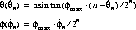
Points on a unit radius sphere are parameterized by two angles, and , using spherical coordinates. is the angle about the Y-axis; is the longitudinal angle from the y = 0 plane. The mapping between rectangular and spherical coordinates is as follows:

(B.1)

Points on the sphere are folded first by octant, and then by sort order of xyz into one of six sextants. All the table encoding takes place in the positive octant, in the region bounded by the half spaces:

This triangular-shaped patch runs from 0 to /4 radians in , and from 0 to as much as 0.615479709 radians in : _max.
Quantized angles are represented by two n-bit integers and , where n is in the range of 0 to 6. For a given n, the relationship between these indices and is

(B.2)

These two equations show how values of and can be converted to spherical coordinates and , which in turn can be converted to rectilinear normal coordinate components via equation B.1.
To reverse the process, for example, to encode a given normal n into and , one cannot just invert equation B.2. Instead, the n must first be folded into the canonical octant and sextant, resulting in n'. Then n' must be dotted with all quantized normals in the sextant. For a fixed n, the values of and that result in the largest (nearest unity) dot product define the proper encoding of n.
Now the complete bit format of absolute normals can be given. The uppermost three bits specify the octant, the next three bits the sextant, and finally two n-bit fields specify and . The three-bit sextant field takes on one of six values, the binary codes for which are shown in Figure B-3.

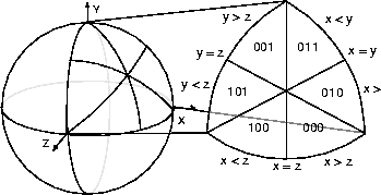
Figure B-3 Encoding of the Six Sextants of Each Octant of a Sphere

This discussion has ignored some details. In particular, the three normals at the corners of the canonical patch are multiply represented (6, 8, and 12 times). By employing the two unused values of the sextant field, these normals can be uniquely encoded as special normals. The normal subcommand describes the special encoding used for two of these corner cases (14 total special normals).
This representation of normals is amenable to delta encoding, at least within a sextant. (With some additional work, this can be extended to sextants that share a common edge.) The delta code between two normals is simply the difference in and : and .

B.9 Modified Huffman Encoding
There are many techniques known for minimally representing variable-length bit fields. For geometry compression, we have chosen a variation of the conventional Huffman technique.
The Huffman compression algorithm takes in a set of symbols to be represented, along with frequency of occurrence statistics (histograms) of those symbols. From this, variable-length, uniquely identifiable bit patterns are generated that allow these symbols to be represented with a near-minimum total number of bits, assuming that symbols do occur at the frequencies specified.
Many compression techniques, including JPEG, create unique symbols as tags to indicate the length of a variable-length data field that follows. This data field is typically a specific-length delta value. Thus the final binary stream consists of (self-describing length) variable-length tag symbols, each immediately followed by a data field whose length is associated with that unique tag symbol.
The binary format for geometry compression uses this technique to represent position, normal, and color data fields. For geometry compression, these <tag, data> fields are immediately preceded by (a more conventional computer instruction set) opcode field. These fields, plus potential additional operand bits, are referred to as geometry instructions (see Figure B-4).
Traditionally, each value to be compressed is assigned its own associated label; for example, an XYZ delta position would be represented by three tag/value pairs. However, the delta XYZ values are not uncorrelated, and we can get both a denser and simpler representation by taking advantage of this fact.
In general, the XYZ deltas statistically point equally in all directions in space. This means that if the number of bits to represent the largest of these deltas is n, then statistically the other two delta values require an average of n - 1.4 bits for their representation. Thus we made the decision to use a single field-length tag to indicate the bit length of X, Y, and Z.
This also means that we cannot take advantage of another Huffman technique that saves somewhat less than one more bit per component, but our bit savings by not having to specify two additional tag fields (for Y and Z) outweigh this. A single tag field also means that a hardware decompression engine can decompress all three fields in parallel, if desired.
Similar arguments hold for deltas of RGB values, and so here also a single field-length tag indicates the bit-length of the R, G, B, and (if present) fields.
Both absolute and delta normals are also parameterized by a single value (n), which can be specified by a single tag.
We chose to limit the length of the Huffman tag field to the relatively small value of six bits. This was done to facilitate high-speed, low-cost hardware implementations. (A 64-entry tag look-up table allows decoding of tags in one clock cycle.) Three such tables exist: one each for positions, normals, and colors. The tables contain the length of the tag field, the length of the data field(s), a data normalization coefficient (the up-shift), and an absolute/relative bit.
The tag field can be 0 to 6 bits in length. Zero-length tags are used when every entry in the table is identical; same data length, same up-shift, and same absolute/relative bit. The tag becomes irrelevant because there is nothing to differentiate. This is probably not all that useful.
One additional complication was required to enable reasonable hardware implementations. As will be seen in a later section, all instructions are broken up into an eight-bit header and a variable-length body. Sufficient information is present in the header to determine the length of the body. But to give the hardware time to process the header information, the header of one instruction must be placed in the stream before the body of the previous instruction. Thus the sequence ... B0 H1B1 H2B2 H3 ... has to be encoded as follows:

... H1 B0 H2 B1 H3 B2 ...

B.10 Geometry Compression Commands
Java 3D's geometry compression protocol defines eight commands to be used in specifying 3D geometry and certain affiliated attributes. This section gives a brief overview of these commands and some of their semantics. More detail of these commands, including their bit layout, is given in the following sections.
vertex
The primary command is vertex. A vertex command always specifies a 3D position, two generalized triangle strip replacement bits (rep), and a mesh buffer push (mbp) bit, and may optionally specify a normal and/or a color. The presence of normal or color data within a vertex command is controlled by two state bits known as the bundling bits: bnv and bcv, respectively.
setNormal, setColor
There are also two stand-alone commands for specifying normals and colors: setNormal and setColor. These commands may be freely interspersed with vertex commands, and semantically have (nearly) the same effect as normals or colors bundled directly with a normal.
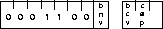
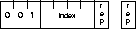
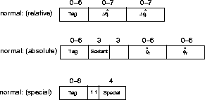
Once a color or normal value is specified, either directly or bundled with a vertex command, that color or normal will remain in effect as the current color or normal until a new value is specified. In this fashion, for example, a constant material color may be specified to apply to a forthcoming sequence of non-color-bundled vertices.
setState
The setState command updates the value of the three state bits. Two of these bits are the normal and color bundling bits; the other one will be described later.
mbr (meshBufferReference)
The meshBufferReference command allows any of the 16 vertices most recently pushed into the mesh buffer to be reused in place of a vertex command at this point. Two vertex replacement bits are also present.
setTable
The setTable command allows a range of entries in one of the three Huffman decompression tables all to be set to the same new value.
passthrough
The passthrough command allows other data to be embedded in the compression stream.
nop
The variable length no-operation nop command allows the compression bit stream to be padded by a specified number of bits. This allows portions of the compression data to be 32-bit aligned when desired.

B.11 Bit Layout of Geometry Decompression Commands
Figure B-4 shows the bit-level layout of the eight geometry decompression commands. Each command has a unique opcode, and then some (possible variable) number of arguments. The actual bit length of many of the components may vary, and if so, a unique (dynamic) Huffman tag at the very start of any variable-length argument delimits the size of the argument.

B.12 Geometry Decompression Command Bit Details
The following subsections describe the bit details of several of the geometry decompression commands, and much of their associated semantics.

B.12.1 nop

The variable length no-operation (nop) command has an 8-bit opcode, a 5-bit count field, and a 0- to 31-bit field of zeros. The total length of the variable-length no-operation command is between 13 and 44 bits.
The variable-length nop command's primary use is to align geometry decompression commands to word boundaries, when desired. This is useful if one wishes to "patch" a decompression instruction in the middle of a stream without having to bit-align the patch.

B.12.2 setState

The setState command has a 7-bit opcode, 3 bits of state to be set, and a spare, for a total length of 11 bits. The first and second state bits indicate if normals and/or colors will be bundled with vertex commands, respectively. The third state bit indicates if colors will contain an alpha value, in addition to the standard RGB. The final state bit is unused, and reserved for future use.

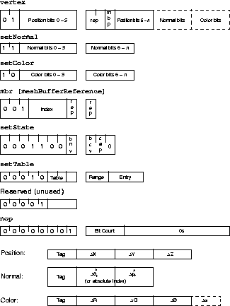
Figure B-4 Bit Layout of Geometry Compression Commands

B.12.3 setTable

The setTable command has a 5-bit op code, a 2-bit table field, a 7-bit address/range field, a 4-bit data length field, an absolute/relative bit, and a 4-bit up-shift field. The total instruction length is fixed at 23 bits. The table and address/range fields specify which decompression table entries to update; the remaining fields comprise the values to which to update the table entries.
The two-bit table specifies for which of the three decompression tables this update is targeted:

00 Position
01 Color
10 Normal
11 Unused-reserved for future use

The seven-bit address/range field specifies which entries in the specified table are to be set to the values in the following fields.

Address/Range Semantics Implicit Tag Length
1a₅a₄a₃a₂a₁a₀ set table entry a₅a₄a₃a₂a₁a₀ 6
01a₅a₄a₃a₂a₁ set table entry a₅a₄a₃a₂a₁0 through a₅a₄a₃a₂a₁1 5
001a₅a₄a₃a₂ set table entry a₅a₄a₃a₂00 through a₅a₄a₃a₂11 4
0001a₅a₄a₃ set table entry a₅a₄a₃000 through a₅a₄a₃111 3
00001a₅a₄ set table entry a₅a₄0000 through a₅a₄1111 2
000001a₅ set table entry a₅00000 through a₅11111 1
0000001 set table entry 000000 through 111111 0

The idea is that table settings are made in aligned power-of-two ranges. The position of the first `1' bit in the address/range field indicates how many entries are to be consecutively set; the remaining bits after the first `1' are the upper address bits of the base of the table entries to be set. This also sets the length of the "tag" that this entry defines as equal to the number of address bits (if any) after the first `1' bit.
The data length specifies how large the delta values to be associated with this tag are; a data length of 12 implies that the upper 4 bits are to be sign extensions of the incoming delta value. Note that the data length describes not the length of the delta value coming in, but the final position of the delta value for reconstruction. In other words, the data length field is the sum of the actual delta bits to be read in plus the up-shift amount. For the position and color tables, the data length values of 1 to 15 correspond to lengths of 1 to 15, but the data length value of 0 encodes an actual length of 16, as a length of 0 makes no sense for positions and colors. For normals, a length of 0 is sometimes appropriate, and the maximum length needed is only 7. Thus for normals, the values 0 to 7 map through 0 to 7, and 8 to 15 are not used.
The up-shift value is the number of bits that the delta values described by these tags will be shifted up before being added to the current value. The up-shift is useful for quantizing the data to save space; it cannot be used to extend the range of the data represented. You are still limited to 16 bits (less for normals) for the resultant data even with a large up-shift value. The up-shift amount is essentially the number of low bits that you don't need to specify in the incoming data as they will always be zero. It is illegal for the up-shift to be greater than or equal to the data length.
So, there are three portions of the resultant data: the sign extension, the incoming data, and the up-shift. For example, if you have a position with a data length of 12 and an up-shift of 4, then the resultant data is made up of 4 sign extension bits in the high bits, 8 bits of incoming data, and 4 bits of zero in the low bits, for the up-shift.
The absolute/relative flag indicates whether this table entry describes values that are to be interpreted as an absolute reference or a relative delta. Note that for normals, absolute references will have an additional six leading bits describing the absolute octant and sextant.

B.12.4 meshBufferReference

The meshBufferReference command has a 3-bit opcode, a 4-bit mesh buffer index field, and a 2-bit vertex replacement field, for a total length of nine bits.
The index specifies which element of the mesh buffer should be used to define the current vertex. A value of 0 indicates to use the most recent vertex that has been pushed into the mesh buffer (before this command). Larger values indicate successively less recent pushes. Only the most recent 16 pushes are addressable.
The two-bit vertex replacement field has the same triangle semantics as it does within the vertex command:

0 0 Restart clockwise
0 1 Restart counterclockwise
1 0 Replace middle
1 1 Replace oldest

There is no mesh buffer re-push bit; mesh buffer contents may be referenced multiple times until 16 newer vertices have been pushed; if a vertex is still needed it must be resent.

B.12.5 Position Subcommand

The position subcommand can only appear within a geometry decompression vertex command, and always as the first subcommand. The tag field can be between 0 and 6 bits in length; all three delta (or absolute) fields will have the same length, between 1 and 16 bits, for a range of lengths between 3 and 54 bits.
As usual, the first six bits of the subcommand are actually forwarded ahead of the rest of the command. Depending on the length of the tag and delta fields, the first 6 bits might only contain the tag, or the tag and some of the X field bits, or any subset up to the entire subcommand, if short enough. However, it is possible for the entire subcommand to be too short. It is not allowed for the tag together with the X, Y, and Z fields to be smaller than the six bits that gets forwarded ahead. There can be no "empty" bits in the forwarded header. If necessary, the tag and/or delta (or absolute) fields must be expanded so that the total number bits used for the entire subcommand is at least six.
For clarity, because it is by far the most typical case, the three coordinate bit fields are labeled X Y Z, though more properly they are X, Y, and Z fields; their actual interpretation is absolute or relative depending on the setting of that bit in the decompression table entry corresponding to the tag field. In both cases the fields are signed two's-complement numbers.
You must always specify at least one absolute position before using any relative positions. It is illegal to have a relative position before the first absolute position.
It appears that, depending on the current position, half of the possible delta values are illegal. (For ease of understanding these examples, we will treat positions as integers.) For instance, going +10,000 from 30,000 will wrap past the positive limit of 32,767 for signed 16-bit two's complement arithmetic. However, this turns out to be very useful. For example, if your current X position is -20,000 and the next X position is 30,000 then the difference that you'd like to use as a delta is +50,000, which is not directly representable. When you compute that difference using 16-bit arithmetic, the value wraps to -15,536, which can be represented as a delta. When -15,536 is added back to -20,000 on decompression, instead of getting -35,536, again the 16-bit arithmetic wraps and we get 30,000, which is the desired result.

B.12.6 Color Subcommand

The color subcommand can appear within either a geometry decompression vertex command or setColor command. The tag field can be between 0 and 6 bits in length; all three (or four) delta (or absolute) fields will have the same length, between 1 and 16 bits, for a range of lengths between 3 and 54 (or 70) bits. As usual, any subcommand with a total length of less than 6 bits has trailing zeros added to pad the length to a minimum of 6 bits.
As usual, the first six bits of the subcommand are actually forwarded ahead of the rest of the command. Depending on the length of the tag and delta fields, the first six bits might only contain the tag, or the tag and some of the R field bits, or any subset up to the entire subcommand, if short enough. However, it is possible for the entire subcommand to be too short. It is not allowed for the tag together with the R, G, and B (and ) fields to be smaller than the six bits that gets forwarded ahead. There can be no "empty" bits in the forwarded header. If necessary, the tag and/or delta (or absolute) fields must be expanded so that the total number bits used for the entire subcommand is at least six.
For clarity, because it is by far the most typical case, the color component bit-fields are labeled R G B (), though more properly they are R, G, and B fields; their actual interpretation is absolute or relative depending on the setting of that bit in the decompression table entry corresponding to the tag field. In both cases the fields are signed two's-complement numbers. A sign bit is required for absolute color components. Negative color components make no sense and are ill-defined, so the sign bit on absolute components should always be zero. Similarly for delta color components, a negative result from adding a delta component to the current component makes no sense, and so negative results are also ill-defined.
If the most recent setting of the cap bit by a setState command is zero, then no fourth (alpha) field will be expected, and must not be present. If the cap bit was set, then the alpha field will be processed and must be present.
You must always specify at least one absolute color before using any relative colors. It is illegal to have a relative color before the first absolute color.
The rest of the graphics pipeline and frame buffer following the geometry decompression stage may choose not to use all (up to) 16 bits of color component information; in this case it is acceptable to truncate the trailing bits during decompression. What the geometry decompression format does require is that color setting of any size up to 16 bits be supported, even if all the bits are not used. Typically, implementations may use just 12 bits, 8 bits, or even 5 bits from each color component.

B.12.7 Normal Subcommand

The normal subcommand can appear within either a geometry decompression vertex command or setNormal command. The tag field can be between 0 and 6 bits in length; the last two angle fields will have the same length, between 0 and 7 bits for deltas and between 0 and 6 bits for absolutes. Six more bits are always present for absolute normals. The range of sizes for a relative normal can be from 6 to 20 bits, and an absolute normal can be from 6 to 24 bits.
As usual, the first six bits of the subcommand are actually forwarded ahead of the rest of the command. Depending on the length of the tag and delta fields, the first six bits might only contain the tag, or the tag and some of the other field bits, or any subset up to the entire subcommand, if short enough. However, in the case of relative normals, it is possible for the entire subcommand to be too short. It is not allowed for the tag together with the delta angle fields to be smaller than the six bits that gets forwarded ahead. There can be no "empty" bits in the forwarded header. If necessary, the tag and/or delta angle fields must be expanded so that the total number bits used for the entire subcommand is at least six.
A normal subcommand is interpreted as relative or absolute depending on the current setting of that bit in the decompression table entry corresponding to the tag field. Unlike the position and color subcommands, the number of fields of a setNormal command differ between the absolute and relative types.
When the subcommand is relative, there are two delta angle fields after the tag field, both of the same length, up to seven bits. These two fields are signed two's-complement numbers. If after delta addition the resulting angle is outside the current sextant or octant, the sextant/octant wrapping rules (described elsewhere) apply. If zero-length angle fields are specified, this is equivalent to specifying a zero value for both fields, i.e., no change from the previous normal. It may be easier to use this method rather than turning off normal bundling for a small number of identical normals.
When the subcommand is absolute, four bit fields follow the tag. The first is a three-bit (fixed-length) absolute sextant field, indicating in which of six sextants of an octant of the unit sphere this normal resides. The second field is also fixed at three bits, and indicates in which octant of the unit sphere the normal resides. The last two fields are absolute angles within the sextant, and are unsigned positive numbers, up to six bits in length. If zero-length angle fields are specified, this is equivalent to specifying a zero value for both fields, i.e., no change from the previous normal. It may be easier to use this method rather than turning off normal bundling for a small number of identical normals.
When the subcommand is absolute, four bit fields follow the tag. The first is a three-bit (fixed-length) absolute sextant field, indicating in which of six sextants of an octant of the unit sphere this normal resides. The second field is also fixed at three bits, and indicates in which octant of the unit sphere the normal resides. The last two fields are absolute angles within the sextant, and are unsigned positive numbers, up to six bits in length. If zero-length angle fields are specified, this is equivalent to specifying a zero for both fields.
You must always specify at least one absolute normal before using any relative normals. It is illegal to have a relative normal before the first absolute normal.
A number of normals lie on the edges or corners where sextants meet (e.g., at = 0 and = 0). You have your choice of multiple sextant/octant pairs that you can use to specify these normals. So choose the sextant/octant that is most convenient for you, usually the one that you can most easily compute deltas from the previous and/or to the following normal.
Fourteen special absolute normals are encoded by the unused two settings within the three sextant bits. This is indicated by specifying the angle fields to have a length of zero (not present), and the first two bits of the sextant field to both have a value of 1. Table B-1 lists the 14 special normals

Table B-1 The 14 Special Normals
Special NX NY NZ Comment
0000 1.0 0.0 0.0 +X axis
0010 -1.0 0.0 0.0 -X axis
0100 0.0 1.0 0.0 +Y axis
0110 0.0 -1.0 0.0 -Y axis
1000 0.0 0.0 1.0 +Z axis
1010 0.0 0.0 -1.0 -Z axis

0001 +X +Y +Z
0011 +X +Y -Z
0101 +X -Y +Z
0111 +X -Y -Z
1001 -X +Y +Z
1011 -X +Y -Z
1101 -X -Y +Z
1111 -X -Y -Z

You cannot specify a delta from a special normal. So, after using a special normal, you must use an absolute normal before using any further relative normals. This can be kind of a pain, so one technique you might want to use is to slightly perturb any normal that would require a special normal subcommand, so that you use an adjacent normal specified by the usual relative normal subcommand. This eliminates the need for breaking up a stream of delta normals with special and absolute normals and most likely will have no visual impact.
The rest of the graphics pipeline and frame buffer following the geometry decompression stage may choose not to use all (up to) 16 bits of normal component information; in this case it is acceptable to truncate the trailing bits during decompression. What the geometry decompression format does require is that normal settings of any size up to 18-bit absolute normals be supported, even if all the decompressed bits are not used.

B.12.8 vertex

The vertex command has a two-bit opcode, a position subcommand (always), a two-bit vertex replacement field, a mesh buffer push bit, and, optionally, a normal subcommand and/or a setColor command, depending on the current setting of the state bundling bits. The two-bit vertex replacement field has the same triangle semantics as it does within the meshBufferReference command:

0 0 Restart clockwise
0 1 Restart counterclockwise
1 0 Replace middle
1 1 Replace oldest

The mesh buffer push bit indicates whether this vertex should be pushed into the mesh buffer so as to be eligible for later re-reference.
The position, normal, and color subcommands have the semantics documented in their individual sections.

B.12.9 setNormal

The setNormal command has a two-bit opcode, and a normal subcommand.
The normal subcommand has the semantics documented in Section B.12.7, "Normal Subcommand."
If a setNormal command is present immediately before a meshBufferReference command, then the new normal value overrides the normal data present in the mesh buffer for that particular mesh buffer reference.

B.12.10 setColor

The setColor command has a two-bit opcode, and a color subcommand. The color subcommand semantics are documented in Section B.12.6, "Color Subcommand."
If a setColor command is present immediately before a mbr (meshBufferReference) command, then the new color value overrides the color data present in the mesh buffer for that particular mesh buffer reference.

B.13 Semantics of Geometry Decompression Commands
The formal semantics of the compression format is best described by a state description of the decompression process. It must be emphasized that these state descriptions are given to show the formal semantics, not an efficient implementation.
The next few sections will present such a state description. While this description is intended to be a complete and unambiguous description of the compression format and decompression semantics, in practice studying both the compression process and the decompression process, and studying code examples for both, is a better approach for the human understanding process.

B.13.1 Header and Body to Variable-Length Command
Geometry decompression commands have a minimum length of eight bits (six bits for subcommands). This allows all geometry decompression commands to be split into two physically separate bit sequences within the compressed stream. The first bit sequence is always of eight bits in length (six for subcommands), the second bit sequence contains the remaining bits of the decompression command (if any). Thus a logical stream of N geometry decompression commands, where each command is split into two bit sequences Hi and Bi (i being from 0 to N - 1) is physically represented as:

H₀ B_-1 H₁ B₀ H₂ B₁ ... H_n-1 B_n-2 H_n B_n-1
OK, so what is this "B_-1"? All compressed geometry sequences have an implied (not physically present) H_-1 of a variable-length no-op opcode, thus B_-1 is always present (starting at the eighth bit of the stream) as any valid variable-length no-op body. (Just five zeros, the minimum-length no-op, is a good default.) Thus the implied no-op opcode "jump starts" the header-forwarded decompression process. This process is reversed at the end of the stream. Hn is a variable-length no-op opcode, but no body is present, as B_n-1 is the last bits of the stream.
This is viable because all compressed geometry streams are presented along with a total bit length of their contents, so no explicit end-of-stream marker is needed. Streams must be rounded up to the nearest full 64-bit word multiple by use of additional variable length no-ops (within the body of the stream, that is, their headers appear before Hn).
This "header-forwarding" shuffled representation is necessary for hardware decompressors to operate efficiently. While this is not an issue for purely software-based decompressor implementations, in order to have one canonical format for both hard and soft decompressors, all decompressors must operate only on the header-forwarded representation; this is the only "official" compression bit-format specified. For a software decompressor, the extra unshuffling adds only slightly to the overall overhead of decompression; for hardware, it is essential.
Thus the first stage in the decompression process is to put the two separate bit sequences for each command back together. The next paragraph describes the flavor of this process, going around the loop approximately one and one-half times. The actual process is more accurately described in state machine semantics.
First the fixed-length eight- (or six-) bit header for the next full command (or subcommand) to be processed is detached from the current head of the compressed stream. Next, the variable-length body bits for the previous command (or subcommand) are detached from the compressed stream and combined with the already extracted header for the previous command; the previous command is now complete and can be processed. Now the fixed-length header for the command after the next is detached from the bit stream, and then finally the variable-length body for the next full command can be detached; the next command is now complete and can be processed.
// pseudocode for converting bitstream into sequences of
// commands

decompress(stream) {
    previous_header <- no-op
    while (not_empty(stream)) {
        current_header <- get_8_bits(stream)
        previous_body <- get_n_bits(stream,
                                        body_length(previous_header))
        process_command(previous_header, previous_body)
        previous_header <- current_header
    }
}
One slight complexity: the get_8_bits() only extracts six bits of header for the color or normal subcommand of a vertex command. It extracts a full eight bits of header in all other cases.

B.13.2 Variable-Length Command to Command
The three decompression tables contain entries for each different numeric tag describing whether the value in the stream is absolute or relative, and length and shift constants describing how to convert the variable-length bit field back into a fixed-length value. The fixed-length value for position and color components is 16 bits in length (sign, unit, 14 fraction); the fields for normal angles are 7 bits (signed), and 3 each for sextant and octant (if present).

B.13.3 Delta Position to Position
absolute_position(x, y, z):
cur_x  x, cur_y  y, cur_z  z
relative_position(x, y, z):
cur_x  cur_x + x, cur_y  cur_y + y, cur_z  cur_z + z
B.13.4 Delta Color to Color
absolute_color(r, g, b {, }):
cur_r  r, cur_g  g, cur_b  b, {cur_   }
relative_color(r, g, b {, }):
cur_r  cur_r + r, cur_g  cur_g + g, cur_b  cur_b + b,
{cur_  cur_ +  }
B.13.5 Encoded Delta Normal to Encoded Normal
State: cur_oct, cur_sex, cur_u, cur_v
absolute_normal(oct, sex, u, v):
cur_oct  oct, cur_sex  sex, cur_u  u, cur_v  v,
relative_normal(u, v):
cur_u  cur_u + u, cur_v  cur_v + v,
if (cur_u < 0)
    cur_u  -cur_u, cur_sex  flip_u[cur_sex]
else if (cur_v < 0)
    cur_v  -cur_v, cur_oct  cur_oct <xor> flip_v[cur_sex]
else if (cur_u + cur_v > 64)
    cur_u  64 - cur_u, cur_v  64 - cur_v,
    cur_sex  flip_uv[cur_sex]

flip_u[6]  = { 4, 5, 3, 2, 0, 1 }
flip_v[6]  = { 2, 4, 1, 1, 2, 4 }
flip_uv[6] = { 2, 3, 0, 1, 5, 4 }
B.13.6 Encoded Normal to Rectilinear Normal
nx  norms[v,u].nx,    ny  norms[v,u].ny,    nz  
norms[v,u].nz,
if (cur_sex & 4) t  nx, nx  nz, nz  t
if (cur_sex & 2) t  ny, ny  nz, nz  t
if (cur_sex & 1) t  nx, nx  ny, ny  t
if (cur_oct & 1) nz  -nz
if (cur_oct & 2) ny  -ny
if (cur_oct & 4) nx  -nx
The contents of the norms[] table is exactly specified, and the next revision of this specification will contain an exact listing of the values.

B.14 Semantics of Vertices
The formal semantics of the vertex processing is best described by a state description of the decompression process. Once again it must be emphasized that these state descriptions are given to show the formal semantics, not an efficient implementation.

B.14.1 Command to Vertex
This section describes the state change semantics caused by each command to generate the next output vertex, prior to assembly into triangles. The internal state consists of the six mode bits, a current normal and current color, normal_override and color_override bits, the 16 mesh buffer vertices, and the current mesh index.
normal(n):
current_normal  n, normal_override  1
color(c):
current_color  c, color_override  1
vertex(rep, mbp, p {, n} {, c}):
current_position  p,
if (bnv) current_normal  n,
if (bcv) current_color  c,
output_vertex(rep, current_position, current_normal, current_
color)
if (mbp) mesh_buffer[oldest_mesh_index].position  p
if (mbp && bnv) mesh_buffer[mesh_index].normal  n
if (mbp && bcv) mesh_buffer[mesh_index].color  c
if (mbp) mesh_index  (mesh_index+1) & 15
normal_override  0, color_override  0
mesh buffer reference(rep, i):
current_position 
            mesh_buffer[(mesh_index - i - 1) & 15].position
if (bnv && !normal_override)
    current_normal mesh_buffer[(mesh_index - i - 1) & 15].normal
if (bcv && !color_override)
    current_color  mesh_buffer[(mesh_index - i - 1) & 15].color
output_vertex(rep, current_position, current_normal, current_
color)
set state(new_bnv, new_bcv, new_cap):
bnv  new_bnv,
bcv  new_bcv,
cap  new_cap,
set table(address, range, entry):
    ...
passthrough(data):
    (null)
vnop(length):
    (null)
B.14.2 Vertex to Intermediate Triangle
This section describes the formal semantics of assembling vertices with replacement commands into nearly finished triangles: the semantics of generalized triangle strips.
output_vertex(restart clockwise, newv):
newest  newv, number_of_vertices  1, ccw = 0
output_vertex(restart counterclockwise, newv):
newest  newv, number_of_vertices  1, ccw = 1
output_vertex(replace_middle, newv):
if (number_of_vertices < 2)
    midlest  newest, newest  newv, number_of_vertices++
else if (number_of_vertices < 3)
    oldest  midlest, midlest  newest, newest  newv,
    number_of_vertices++,
    intermediate_triangle(ccw, oldest, midlest, newest)
else if (number_of_vertices == 3)
    midlest  newest, newest  newv,
    intermediate_triangle(ccw, oldest, midlest, newest)
output_vertex(replace_oldest, newv):
if (number_of_vertices < 2)
    midlest  newest, newest  newv, number_of_vertices++
else if (number_of_vertices < 3)
    oldest  midlest, midlest  newest, newest  newv,
    number_of_vertices++,
    intermediate_triangle(ccw, oldest, midlest, newest)
else if (number_of_vertices == 3)
    oldest  midlest, midlest  newest, newest  newv,
    ccw = 1 - ccw,
    intermediate_triangle(ccw, oldest, midlest, newest)
B.14.3 Intermediate Triangle to Final Triangle
The final stage is to take into account the current rnt and rct mode bits settings. These control the semantics of the normal and color vertex data. The semantics of the counterclockwise bit also can be expressed here; thus, the final triangles can always be assumed to be front facing when their vertices appear in counterclockwise order.
intermediate_triangle(ccw, v1, v2, v3):
if (ccw)
    final_triangle(v1.position, v1.normal, v1.color,
                     v2.position, v2.normal, v2.color,
                     v3.position, v3.normal, v3.color)
else if (!ccw)
    final_triangle(v2.position, v2.normal, v2.color,
                     v1.position, v1.normal, v1.color,
                     v3.position, v3.normal, v3.color)
B.15 Outline of Geometry Process
Java 3D only formally defines the geometry compression format and the decompression semantics. Authoring tools are free to employ whatever geometry compression algorithms they choose, as long as the results adhere to the specifications described in the previous sections.
However, to further document the semantics of the geometry compression format, an overview of one particular geometry compression algorithm is given here.

B.15.1 Compressing Geometry Data
Group the geometry to be compressed into separate rigid objects. Typically such objects will be individually culled during rendering, so you should not join objects too extensively prior to compression. In optimized systems, the granularity of object splitting will be computed by an algorithm that takes culling optimization into account.

B.15.2 Convert to Generalized Mesh Format
Once a group of geometry has been identified, it is next converted into generalized mesh format. This is a complex step, and a number of topological analysis-based algorithms have been applied to it.
The next step is the quantization of the geometry positions, colors, and/or normals. All these quantizations can be varied within the geometry, but for simplicity a single fixed quantization of each is assumed here.

B.15.3 Position

Normalize the position data.
The containing bounding box for the object is computed. This is the minimal box such that all geometry vertices are contained within it. The vertices are then all normalized to be contained within this bounding box by first subtracting the XYZ location of the bounding box center from the vertex XYZ and then dividing all the XYZ vertex values by the half length of the longest side of the bounding box. Thus all normalized positions will be within the ±1 unit cube. A constant matrix transform corresponding to an offset to the center of the bounding box, and an inverse scale by the half length of the longest side of the bounding box are created as a prologue for the geometry data.

Quantize the position data.
Assuming that position data is to be quantized to n bits, each vertex position component should be multiplied by the value of 2n and then rounded to the nearest integer.

B.15.4 Normals

Normalize the normals.
Each normal should be normalized to unit length.

Quantize the XYZ components of the normal to 14 bits accuracy
Each normal component should be multiplied by 2¹⁴, rounded to the nearest integer, and then converted back to floating-point representation and divided by 2¹⁴.

Quantize the XYZ components of the normal to 14 bits accuracy
If an XYZ component of the normal is negative, invert it and save the original sign bits as a three-bit octant value:
oct = 0;
if(nx < 0.0) oct |= 4, nx = -nx
if(ny < 0.0) oct |= 2, ny = -ny
if(nz < 0.0) oct |= 1, nz = -nz
Fold the normal to the nX > nZ > nY sextant
Check (in exactly the following order):
sex = 0;
if (nx < ny) t = nx, nx = ny, ny = t, sex |= 1
if (nz < ny) t = ny, ny = nz, nz = t, sex |= 2
if (nx < nz) t = nx, nx = nz, nz = t, sex |= 4
Match the nearest quantized normal representation
Take the dot product of the normal with each of the quantized reference normals in the table for the specified number of quantized normal bits. That UV normal index for the reference normal that gives the greatest (nearest unity) dot product result is the new quantized normal representation (along with the octant and sextant representation).

Check for special normals

B.15.5 Colors
The colors are assumed to be in a 0.0 to 1.0 representation to begin with.

Quantize the color values.
Assuming that color data is to be quantized to n bits, each vertex color component (R, G, B, and optionally ) should be multiplied by the value of 2n and then rounded to the nearest integer.

B.15.6 Collect Delta Code Statistics
Make a pass in generalized mesh order through all vertices in the geometry. For each successive pair of vertices, compute the difference between their component values, compute the bit length of this (signed) difference, and histogram this bit length. Specifics for each component type are detailed in the next sections.

B.15.7 Position Delta Code Statistics
Compute X, Y, and Z. Determine which of these has the greatest magnitude. Compute the number of bits for this component, including one sign bit. This is the length to be histogrammed for positions.

B.15.8 Color Delta Code Statistics
Compute R, G, B, and (if present). Determine which of these has the greatest magnitude. Compute the number of bits for this component, including one sign bit. This is the length to be histogrammed for colors.

B.15.9 Normal Delta Code Statistics
For a given pair of normals, check to see if they have the same octant and sextant. If so, compute U and V. Determine which of these has the greatest magnitude. Compute the number of bits for this component, including one sign bit. This is the length to be histogrammed for this pair of normals.
If the normals have different sextants and/or octants, check to see if their sextants share an edge. Depending on what type of edge they share, the delta including the change in edges is encoded in one of three ways: U + U < 0, V + V < 0, and U + U + V + V > 64. Each case is discussed in the paragraphs below. The sextant numbers are from the binary codes shown in Figure B-3.
Sextants 0 and 4, 1 and 5, and 2 and 3 share the U = 0 edge. When crossing this boundary, U becomes ~U - last_u. This will generate a negative cur_u value during decompression, which causes the decompressor to invert cur_u and look up the new sextant in a table.
Sextants 0 and 2, 1 and 3, and 4 and 5 share the U + V = 64 edge. U becomes 64 - U - last_u and V becomes 64 - V - last_v. When cur_u + cur_v > 64, the decompressor sets cur_u = 64 - cur_u and cur_v = 64 - cur_v, and a table lookup determines the new sextant.
Each sextant shares the V = 0 edge with its corresponding sextant in another octant. When in sextants 1 or 5, the normal moves across the X-axis, across the Y-axis for sextants 0 or 4, and across the Z-axis for sextants 2 or 3. V becomes ~V - last_v. The decompressor inverts a negative cur_v and performs a table lookup for a mask to exclusive-OR with the current octant value.
Otherwise the normals cannot be delta encoded, and so the second (target) normal must be represented by an absolute reference to its three octant, three sextant, and 2 N-bit U V addresses. This is the length to be histogrammed for this pair of normals.

B.15.10 Assign Huffman Tags
Encode data into variable-bit length decompression commands.
One can use an algorithm similar to the one used by the JPEG image compression standard. The main differences are how codes are reassigned when their lengths exceed the maximum code length and how the data bits are encoded in the compressed data stream.
The frequencies of the data lengths are used as leaf nodes in a binary tree. The algorithm used to generate the tree places the less frequent codes deeper in the tree. After the tree is built, the traversal path to a leaf node becomes its Huffman code, and the depth in the tree becomes its code length.
Codes generated with a length greater than six, the maximum code length, must be shortened. These nodes are merged with more frequent nodes by increasing the number of sign bits included with the smaller data length.

B.15.11 Assemble the Pieces into a Bit Stream
Given the sequence of variable-bit-length decompression commands, shuffle the first eight (six) bits of each command ahead of its predecessor's body.

Java 3D API Specification

¹ Deering, Michael. "Geometry Compression." Computer Graphics Proceedings, Annual Conference Series, 1995, ACM SIGGRAPH, pp 13-19.
Copyright © 1998, Sun Microsystems, Inc. All rights reserved.

Address/Range	Semantics	Implicit Tag Length
1a₅a₄a₃a₂a₁a₀	set table entry a₅a₄a₃a₂a₁a₀	6
01a₅a₄a₃a₂a₁	set table entry a₅a₄a₃a₂a₁0 through a₅a₄a₃a₂a₁1	5
001a₅a₄a₃a₂	set table entry a₅a₄a₃a₂00 through a₅a₄a₃a₂11	4
0001a₅a₄a₃	set table entry a₅a₄a₃000 through a₅a₄a₃111	3
00001a₅a₄	set table entry a₅a₄0000 through a₅a₄1111	2
000001a₅	set table entry a₅00000 through a₅11111	1
0000001	set table entry 000000 through 111111	0

0 0	Restart clockwise
0 1	Restart counterclockwise
1 0	Replace middle
1 1	Replace oldest

Special	NX	NY	NZ	Comment
0000	1.0	0.0	0.0	+X axis
0010	-1.0	0.0	0.0	-X axis
0100	0.0	1.0	0.0	+Y axis
0110	0.0	-1.0	0.0	-Y axis
1000	0.0	0.0	1.0	+Z axis
1010	0.0	0.0	-1.0	-Z axis

0001				+X +Y +Z
0011				+X +Y -Z
0101				+X -Y +Z
0111				+X -Y -Z
1001				-X +Y +Z
1011				-X +Y -Z
1101				-X -Y +Z
1111				-X -Y -Z