
by
Douglas A. Lyon
A Thesis Submitted to the Graduate
Faculty of Rensselaer Polytechnic Institute
in Partial Fulfillment of the
Requirements for the Degree of
DOCTOR OF PHILOSOPHY
Major Subject: Computer and Systems Engineering
Approved by the
Examining Committee:
___________________________________
George Nagy, Thesis Adviser
___________________________________
Frank DiCesare, Member
___________________________________
Robert Kelley, Member
___________________________________
Bruce Piper, Member
Rensselaer Polytechnic Institute
Troy, New York
December 1991
Contents
2.4-1 Sensor Taxonomy. 23
2.4.1-1 Critical Angle of Sonar. 25
2.4.1-2 A Multi-element Ultrasonic Ranging Array. 26
3.1-1 Parking Constraints. 35
3.1.2-1 Family of Fifth-Order Polynomials and Respective Curvatures. 39
3.2.1-1 2-D Car States. 42
3.2.1-2 The Turning Radius of the Car. 44
3.2.2-1 Example Maneuver 46
3.2.2-2 Example Angles and Curvature 47
3.2.2-3 Maximum Y-Deflection vs PSL-L. 48
3.2.2-4 Y-Deflection vs PSL-L. 49
4-1 Open-loop Control. 51
4.1.1-1 Error-Free Control. 52
4.1.2-1 Graph of 1-D Motion. 55
4.1.3-1 Open-loop Control using a Plant Model with Error. 56
4.1.3-2 Underestimation of Acceleration. 60
4.1.3-3 Overestimation of Deceleration. 61
4.1.3-4 Underestimation of Acceleration and Overestimation of Deceleration. 62
4.1.3-5 Summary of Open-loop Errors. 63
4.2.2-1 Error-Free Curvature Tracking. 71
4.2.2-2 Angular Acceleration. 72
4.2.3-1 Open-Loop Control with 25% Underestimation. 74
5.1-1 Closed-loop Control. 77
5.2.1-1 Internal Sensor Feedback. 79
5.2.3-1 Internal and External Sensors. 82
5.2.4-1 Comparison of 1-D Control Regimes. 84
5.2.4-2 A Single Maneuver and 1-D Control Regimes. 87
5.3.1-1 Dead Reckoning. 90
5.3.2-1 External Sensors in 2-D. 91
5.3.3-1 Internal and External Sensors Used by the Observer. 92
5.3.3-2 The Observer's use of the External Orientation Sensor. 93
5.3.3-3 The Observer's Estimate of Speed. 94
5.3.3-4 The Observer's Estimate of Path length. 95
5.3.4-1 Comparison of 2-D Control Regimes. 97
5.3.4-2 Multiple-Maneuvers and 2-D Control Regimes. 100
A.3-1 Ten Maneuvering Curves. 134
A.3-2 Ten Curvature Curves (k(u) vs u). 135
A.3-3 Derivative of the Curvature Function. 135
A.3-4 Family of Fifth-order Polynomials. 136
B-1 A Wheel Perpendicular to a Plane. 138
D-1 The Four Basic Modeling Primitives. 142
D.1-1 Second Order Harmonic Oscillator. 145
D.1-2 A Second Order Harmonic Oscillator. 146
D.2-1 A Model of a Non-Linear 2nd-Order Differential Equation. 147
D.2-2 Graph of Stochastic Non-linear, Coupled-Differential Equations. 148
D.5-1 1-D Plant Model with Longitudinal Controller. 155
D.5-2 The STELLA Diagram of the Plant. 156
D.5-3 The Reference Path Generator, Steering Controller and Plant Model. 157
D.5-4 Sensors, Clocks and Fusion. 158
D.5-5 Feedback Mode Logic, the Control Panel and Fusion. 159
D.5-6 1 and 2-D Sensor Fusion in the Observer. 160
E-1 Summary of the L1 Errors for Various Mix Ratios 168
F-1 PSL-L vs Measured Maneuver Room. 169
G-1 Linear Acceleration vs Steering Speed. 171
H-1 Modeling Error vs Plant Performance. 173
First and foremost among them has been George Nagy, my thesis advisor. I wish to express my sincere gratitude to George Nagy, for the advice, encouragement and support that he provided during the years I have spent at Rensselaer.
Special thanks go to Tom DeWitt, for his commentary, technical assistance and for his tireless reading of drafts of the thesis.
I thank all my committee members for providing the guidance and direction that allowed me to develop this work.
I thank Jim Modestino for providing financial support during the doctoral research.
I thank all the members of the IPL for making the lab an enjoyable place to work.
My father and mother, Martin and Rheva Lyon, have supported me with their love, advice and money during the four and one half years it has taken to complete this research. Without their encouragement and support I would have been unable to compete this thesis.
A short parking space requires multiple reversals of direction. Several s-shaped curves are compared using the rate at which the car approaches the curb as the objective function. A fifth-order parking polynomial is found to dominate the other curves in curvature-constrained docking maneuvers.
An odometer, a steering-wheel angle meter, an orientation sensor and an absolute position sensor enable correction of car-model error. The sensors' reliability is inversely related to their availability. The 20 sample-per-second internal sensors - the odometer and the steering-wheel angle meter - give the observer the ability to perform dead-reckoning with 10% measurement error. The external sensors - the orientation meter and the absolute position sensor - are error-free but can be sampled only 5 times per second.
Both ad-hoc logic and nonholonomic constraints are used to perform sensor fusion. The combination of external and internal sensors outperforms either. Each by itself is, however, superior to open-loop control using only the observer's model.
Bang-bang control is used to change the steering-wheel angle and the drive-train. Control of these variables allows the car to attain any feasible configuration. Accelerations are piecewise constant, and velocity is unconstrained. Proportional plus derivative control is used to formulate the bang-bang control. The coefficients of the control equations are found by experiment. Although the trajectory of the rear wheel is prescribed by the parking polynomial, only the front wheel is subject to direct control.
All simulations are performed with STELLA(TM) (Structured Thinking Experimental Learning Laboratory with Animation). STELLA allows interactive set up and simulation of nonlinear, coupled, initial boundary value problems. Some symbolic manipulations are performed with MAPLE(TM).
In order to formally state the problem, several assumptions are made. We assume that the car is capable of autonomous control. For autonomous control to be possible, the car must have sensors, effectors and sufficient on-board computing power to run the parking program in real time.
The sensors must have some error and the nature of the error is assumed unknown. Further, the worst-case error for the sensors is assumed to be systematic error. We assume that there are two kinds of sensors, internal and external, and that these sensors have an availability which is inversely related to their reliability. The sensors are sampled at known rates.
There are two effectors in the car, one controls the 1-D motion, the other controls the steering. We assume that the car steers with its front wheel and that it has a limited turning radius. There are also limits on the car's 1-D and steering accelerations. The limits on acceleration and turning radius are assumed to be known. It is assumed that the front of the car follows the front wheel without slip, and so the car is subject to nonholonomic constraints. We assume that the rear wheel remains parallel with the main axis of the car. No provisions are made to model the differential coupling in the drive train or the width of the car: the model is essentially that of a motor cycle.
The parking program is assumed to be capable of performing control using the measurements provided by the sensors to alter effector commands. The program contains a model of the car and it is assumed that this model has error.
The parking space is assumed to be well approximated by a U-shaped rectangle. The dimensions of the space are assumed to be known, without error, to the parking program. For the purpose of control and comparison, it is assumed that the distance to parking space curb is not a factor.
Given a car in a parking space with discrete sensor feedback, and modeling errors in acceleration, car inertia and steering inertia, subject to nonholonomic and kinematic constraints (curvature and acceleration), develop a program that minimizes the time to park the car.
The path which the car follows is designed and tested against other paths. Several s-shaped curves are compared using the rate at which the car approaches the curb as the objective function. A fifth-order parking polynomial is found to dominate the other curves in curvature-constrained docking maneuvers. It is known that the rear of the car must follow this path and that the steering-wheel angle may be computed for any point on the path.
In the simulator we have two models of the car, the plant and the plant model. The plant is an error-free model of the car and is used to determine the actual motion of the car. The plant model is an erroneous model of the car and is used to show the worst-case control scenario and to show the effect of sensor fusion on control. The sensors are modeled in the simulator and they measure the plant-states with systematic error.
The plant model is a part of a subsystem called the observer. The observer's function is to perform sensor fusion to provide plant-state estimates for the controller. The observer can access the plant model at any time during the simulation but its access to the plant is restricted by the sensors and their error.
The controller is a subsystem which issues bang-bang control commands which change 1-D and steering acceleration. Accelerations are piecewise constant, and velocity is unconstrained. Proportional plus derivative control is used to formulate the control decisions. Experiments are used to find the coefficients of the control equations.
The parking problem is a special case of goal-directed motion of an autonomous land vehicle. There are constraints on rotation, velocity, acceleration and collision. A solution to the parking problem has significant implications for factory-floor motion planning. For example, the use of automated vehicles for moving parts is becoming common. These vehicles follow predefined paths that are inflexible. Motion-planning research, presented here, has a major impact on the range of use of these vehicles.
Other applications of this research include autonomous-motion planning and computer animation. Autonomous-motion planning is a requirement of vehicles which cannot be operated remotely, as happens over great distances (i.e., a planetary rover). Computer animation makes use of this work by providing high-level goal-directed motion specification to an animation programmer.
Automation helps to eliminate human error and make operations efficient. It also insures safe, well-constrained operation while providing high-level motion specification.
Chapters 3 addresses the problem of static curvilinear path generation for parking. A curve for parking a car is derived and examples are shown. Constraints on the curve include initial and final position, orientation and curvature. There is also a constraint on the global curvature extrema; a fifth-order polynomial results. To track the fifth-order polynomial's curvature, the relationship between the curvature of the back and the front of the car is developed. This leads to the introduction of the nonholonomic constraints on the car. The rest of the thesis addresses the problem of tracking the curves under dynamic conditions.
Chapter 4 summarizes a study of open-loop bang-bang control in 1-D and 2-D. The open-loop control with plant-model error establishes a worst-case performance on control. The open-loop control with no plant-model error establishes a best-case performance on control. The bounds are used in a comparative study in Chapter 5.
Chapter 5 summarizes a study of closed-loop bang-bang control in 1-D and 2-D. New sensor fusion techniques are developed which use sensors whose reliability is inversely related to availability.
Chapter 6 summarizes the results found in the thesis and discusses topics for future research.
Appendix A provides a derivation of the fifth-order polynomial using a computer generated proof. A symbolic manipulation program (called Maple) generates FORTRAN code that will compute the fifth-order polynomial in minimum computer time.
Appendix B defines holonomic and nonholonomic systems.
Appendix C shows that the effect of rolling resistance on the model developed in Chapter 4 is negligible.
Appendix D describes the use of STELLA (Structural Thinking and Experimental Learning Laboratory with Animation) for modeling and simulation. Non-linear, time-varying systems may be represented with a small set of graphical primitives and formulae. There are examples with complex deterministic and stochastic relationships.
Appendix E contains a summary of simulation performed with different proportional and derivative control mix ratios.
Appendix F provides experimental data which allows the measured maneuver room to be mapped into the PSL parameter which takes into account the worst-case plant-model error. This reduces the chance that overshoot will result in a collision.
Appendix G examines the effect of changing the linear acceleration of the car on the speed needed to steer it.
Appendix H compares various modeling errors in the plant model with tracking performance.
Appendix I contains a glossary of symbols and terms used in the thesis.
The rest of this chapter covers six categories of parking literature: legislation on parking, planning, control, sensors, sensor-data fusion and procedural knowledge representation.
The space-allocation literature establishes guidelines for car and parking-space geometries. Much of the space-allocation literature is old and out of date. This is due to the rise in the number of small cars. In 1950, for example, the recommended parking space was 2.4 meters wide and ranged from 6.1 to 6.7 meters in length [Bair 1950]. Seven years later this recommendation was unchanged [Ricker 1957]. Small car-parking stalls are now less than 2.4 meters wide and less than 4.6 meters long. The increase in the number of small cars has led to a 20% increase in the number of small parking spaces since 1978. Cars currently range in size from under 1.6 meters in width and 4.3 meters in length to over 1.9 meters in width and 5.5 meters in length. Further, turning radius (as defined in this thesis) varies from 2.4 meters to 3.6 meters [Weant 1985]. Therefore, any realistic parking algorithm must accommodate different car and parking dimensions.
The STRIPS model was one of the first applications of forward production [Fikes and Nilsson 1971]. In the STRIPS model the world consisted of blocks that could be moved around by a simplified robot hand. Blocks could be cleared, placed on top of each other and the robot hand could be emptied. Several precondition formulas (used as implicational rules) constrained production-rule firing. A database described the world to which additional structures were appended. Forward production rules modeled robot actions which altered a global database [Nilsson 1980].
The STRIPS approach generates plans in advance but error in execution can cause plan failure. Improvement is obtained by applying partially executed, and previous plans, via plan splicing or dynamic replanning. These techniques provide an error execution recovery scheme [Vere 1985] [Porta 1986].
Domain specific knowledge must be incorporated in any planner that plans for real-world problems on a local level.
Shortest-path planning algorithms find a collision-free minimum path for a body among obstacles. The shortest-path planning problem is a harder problem than the path-planning problem. Ackman proves that the shortest-path planning is an NP-Complete (Nondeterministic Polynomial) problem of O(2n), where n is the number of objects [Ackman 1985].
There has also been work in the reduction of path-planning to a problem of search. One approach uses a digitized-terrain map to weight a grid representation. Weights penalize elevation, mobility, cultural features and military threats. A search through the grid develops a path [Mitchell and Keirsey 1984]. There are also algorithms that plan on multiple levels. In one instance, there are three levels that use varying abstraction: a mission planner, a long range planner and a local planner. These planners plan for mission goals, long-range paths and obstacle avoidance [Mitchell et al. 1984]. With respect to the multiple-level planning, a local planner solves the parking problem.
A design technique using varying levels of abstraction is shared by a field called intelligent control and this will be considered in Section 2.3.
Another method of planning with error is dynamic replanning. Dynamic replanning allows relaxation of implicit assumptions made by SPAR. Apriori knowledge of goals is not always a reasonable assumption. When this assumption is relaxed, SPAR (and static planners) will fail. Another assumption is that events are on time. SPAR generates check-points and contingency plans for on-line execution [Porta 1986]. Excellent arguments, based on computation limits, may be advanced to support this type of planning. In the parking problem, sensor data may be sampled slowly. Local control of a correctly modeled system may be better effected by classic control techniques.
Kinodynamic constraints are a combination of dynamic constraints (i.e., force, velocity and acceleration bounds) and kinematic constraints (i.e., collision avoidance). Time-optimal kinodynamic solutions have expanded their sense of optimality from min-time to both min-time and safe obstacle avoidance margins [Donald et al. 1989].
The autonomous land vehicle literature addresses the maneuvering of a point object in a weighted terrain, or the motion of a vehicle without parking constraints [Mitchell et al. 1984]. This literature is not directly applicable to automating the parking process.
There is literature on mathematical modeling of the car suspension and outside forces during car motion [Speckhart 1973] [Yamada et al. 1967]. The models are complex and must be augmented for path generation. They consider the bounce, pitch and roll motions of a sprung mass. It is beyond the scope of this thesis to address a model of this complexity (which calls for dynamical equations of motion with more than six degrees of freedom).
Recent spatial-reasoning research has addressed the nonholonomic constraints that have plagued people since the invention of the cart [Edelen 1977]. One solution is based on a configuration-space approach [Latombe 1989]. Using the nonholonomic constraints (see Appendix B for a definition), it is possible to establish a configuration space which may be searched more efficiently than an unconstrained space [Laumond et al. 1988]. Using these techniques, as pointed out by Tournassoud, the motion-planning problem is divided into the "local" and "global" planning subproblems in a manner similar to Brook's approach [Brooks 1982] [Tournassoud 1988]. The nonholonomic find-path algorithm is able to solve the nonholonomic-docking problem as a subproblem. The configuration-space solutions to the find-path problem do not address the reduction of the number of maneuvers and this is an important open problem [Tournassoud 1988]. We have not found any previous solution to the nonholonomic find-path problem in an uncertain configuration-space.
The parking problem has been reduced to a problem of search of the configuration space by assigning metric weights based on obstacle proximity. A path was derived based on the contribution of the weight to an equipotential field. This approach is excellent for path generation, particularly for safe paths, but does not consider the curvature constraints inherent in parking a car [Dorst and Trovato].
Intercept control is a kind of spatial reasoning which uses homogeneous coordinate transformations and numerical methods to minimize the time to intercept a target. The homogeneous coordinate transformations rotate and translate the interceptor relative to the target. This has some application in the area of car parking. For example, when a car turns about its center, the intercept-control approach can be used to determine when a collision will occur. When a car is pulling into a space, intercept control determines when to straighten out to avoid mounting the curb.
There are concepts surrounding the intercept-control work that pertain only to the intercept problem. Details may be found in [Burke 1975] [Real et al. 1986].
Plato is credited with the earliest thoughts about feedback in his approach to economic regulation, but perhaps one of the first practical uses of feedback was in the regulation of the speed of Watt's steam engine in 1789 [Bennett 1979]. The 150-year phase (from 1790 to 1940) which followed the steam engine regulation problem was characterized by practical engineers solving problems which were beyond their theoretical understanding. Theory began to have useful applications during World War II where the need for high-speed servomechanisms became acute [Bennett 1979].
The practical approaches to control which engineers have considered between the time of Plato and about 1930 are beyond the scope of this literature review. We can credit these early engineers with creating the need for a theory which could explain their solutions. If practical engineers waited for theoretical understanding to solve a problem, we might be wearing bearskins instead of beepers.
The post-1930 control literature may be divided according to the taxonomy which is shown in Figure 2.3-1. Control literature taxonomy has been complicated with the advent of interdisciplinary approaches. The field of systems science is one such example. It arises as a merger between artificial intelligence and automatic control. In one approach, three collaborating expert systems replace the classical plant/compensator control loop [Lirov et al. 1988]. The heavy reliance upon heuristics in such an approach appears to make it lie in classic control; however, the use of the expert system is new and places the approach in the field of intelligent control.

Figure 2.3-1. Post-1930 Control Literature Taxonomy.
The control literature taxonomy has been complicated by interdisciplinary approaches.
Classical control theory was developed between the 1930's and the 1960's. These techniques include stability theory, transformation techniques and heuristic intuition [Tse et al. 1989]. In classic control, direct methods are used to formulate the control law in order to ensure that each of the design constraints is satisfied [Safonov et al. 1977].
Classical stability theory and frequency-response analysis provides desired stability and performance by manipulation of poles and zeros. This is a mature theory when dealing with linear systems [Hung et al. 1952]. When considering the stability and frequency response of non-linear equations the analysis is more complex. This theory is not as mature as the linear control theory [Lukes 1982].
Modern control theory uses a variety of mathematical disciplines: optimization, calculus of variations, combinatorial search, etc. Modern control system designs are based on models of the plant and the sensor feedback. Uncertainty can create inefficient control designs. Poor or inefficient modeling of the operating environment and sensor error are sources of uncertainty. While a precise strategy for reaching a goal may be known, the relative position and orientation of the car is imperfectly known. In addition, the dimensions of the objects in the environment and therefore the precise target area are imperfectly known [Farreny et al. 1986].
Modern control is based on a body of knowledge called feedback control theory [Ralston et al. 1983]. The parking problem has been formulated with nonholonomic constraints (see Appendix B) and accurate models must therefore be non-linear. Modern control offers numerical methods and search techniques as a means for finding a control solution [Westcott 1969]. However, this approach is too complex to be solved on-line since searching a nonholonomically constrained configuration-space requires considerable computational resources[2] [Barraquand et al. 1989].
There are some analytic solutions to nonlinear systems. For example, Pontryagin's minimum principal has been applied to a class of nonlinear PDE systems [Huang et al. 1989]. However the systems were only quadratic and 2-D.
Intelligent control is the discipline that designs Intelligent Machines to perform anthropomorphic tasks with minimum supervision and interaction with a human operator. It may involve elements of three different disciplines: artificial intelligence, operations research and system theory [Valvanis 1986]. It is difficult to apply classical control techniques of stability analysis and frequency response to intelligent control solutions, but the application of intelligent control has inspired new research in the area of non-linear adaptive control.
Intelligent machines are hierarchical structures organized according to the Principle of Increasing Intelligence with Decreasing Precision [Saridis 1988]. For example, the organization level performs information-processing tasks in association with a long-term memory, the coordination level deals with specific information-processing tasks with a short-term memory only, and the execution level performs the execution of tasks through hardware using feedback control methods [Saridis 1990].
Before the design of the control, the state variables, input, model, feedback and goals must be known [Meystel Preprint]. Relaxation of this assumption places us in an area that lies between artificial intelligence and control system theory. There has been work unifying artificial intelligence and control resulting in a hierarchic control approach [Kyriakopoulos 1991]. Search techniques in path-planning involve a generate-and-test approach [Bonner et al. 1989].
Fuzzy logic control is another kind of modern control which can control non-linear systems [Mamdani et al. 1984]. Farreny and Pradre design their fuzzy controller under the assumption that the car moves so slowly that control lag is negligible[3] [Farreny et al. 1986]. Their approach is to use linguistic rules to perform high-level planning. Sugeno takes a fine motion control approach to the formulation of the fuzzy rules for parking [Sugeno et al. 1985].
The Farrenny and Pradre approach to describe the rules linguistically has a linguistic approximation drawback. Suppose the knowledge engineer asks "How much laundry do you have?" The answer of "Oh, just a little." involves qualitative linguistic terms whose meaning is difficult to quantify. If the expert does not own a washing machine and dislikes doing laundry, there may be a mere eight to ten loads. Relative terms cause uncertainty. Perhaps relative terms should not be used when quantities are known with certainty.
Neural nets contribute another approach to non-linear control [Anderson et al. 1989]. The adaptive part of the neural network indicates that there are parameters requiring no precomputation and are formulated by a learning algorithm. A drawback of this method is that thousands of training sessions are needed to "teach" the network how to park [Widrow et al. 1990].
In summary, there are two intelligent control approaches to parking; fuzzy control and neural network. The advantage of the fuzzy control approach is that it deals directly with uncertainty in the parking problem [Farreny et al. 1986]. There are disadvantages to fuzzy parking control: it may be difficult for the operator to verbalize the knowledge, it is very difficult to give general design procedures, the operator's skill is important, and the control results will not be better than the operator's. In addition, published results show parking failures. These failures of fuzzy control are attributed to sensing and speed-control errors, the very errors which fuzzy control is supposed to deal with [Sugeno et al. 1985]. The advantage of the neural network approach is that it is self-learning and that it too deals directly with uncertainty in the parking problem. The disadvantages to the neural network approach are that the operator's skill is important, the control results will not be better than the operator's and tens of thousands of lessons are needed to train the controller [Widrow et al. 1990].
Modern control has made progress in the area of linear systems [Lewis 1986]. In order to use the theory of linear systems, linear approximations must be made on point-to-point motion between sensor samples. For example, in the Kalman filter, possible parameter variations are computed using recursive least-squares-estimation algorithms [Durieu et al. 1986].
The Kalman filter is a kind of optimal estimator which grew from the optimization theory branch of modern control (see Figure 2.3-1). The Kalman filter uses a linear quadratic regulator (LQR) formulation to estimate the state of a system. The LQR contains a linear model of the system to be regulated. In the case of a non-linear system, the LQR's model must be a linear approximation. The LQR also contains a quadratic penalty function and this is formulated using the value of the square of the deviation between the state of the system and the estimate of the system's state [Young 1969]. To make the computation tractable, it is assumed that the noise statistics are known a priori and that sensors are uniformly sampled. Non-uniform sensor sampling of a non-linear system with unknown noise statistics represents a significant relaxation of the assumptions made by the Kalman filter approach [Maybeck 1990].
A current trend in robotics is to perform off-line planning followed by on-line trajectory tracking. This reduces the dynamic path-planning problem to static path-planning followed by tracking [Sing 1989].
Tracking without noise is a problem that may be solved using modern control techniques [Athens and Falb 1966]. When sensors provide incomplete information a reduced-order observer can be used to provide an estimate of the state of the plant. If the sensor noise is Gaussian and the system is linear, the Kalman filter is a provably optimal estimator. To extend the Kalman filter's abilities beyond the linear system, one may be tempted to merge the Kalman filter with an intelligent controller; however, this makes a complex and poorly understood system.
Several devices are able to acquire range data. There are two basic categories of range-finding devices: direct and indirect. Indirect devices include stereoscopic vision and swept-focus; direct devices include diffraction profilometry [DeWitt 1987], ultrasonic [Polaroid] [Texas Instruments], RADAR and LADAR technologies [Wesolowicz 1987]. The relationship of these sensors to one-another is shown in Figure 2.4-1 [Ruocco 1987].
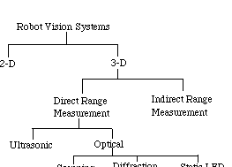
Figure 2.4-1. Sensor Taxonomy.
While optical range measurement technologies yield superior accuracy, ultrasonic sensors are inexpensive, small and in common use.
In general, radar systems are more difficult and more expensive to produce than sonar [Hovanessian 1988]. For this reason the radar approach has not been given full consideration.
Determining path-length is easier than determining range since high-accuracy odometers are available. If multispeed pancake synchros are used, accuracies of arc-seconds can be obtained [Diermengan 1990][4]. Due to the availability of excellent odometers we do not consider odometer sensor error directly. We do model tire slippage, however.
Wide-beam sonar systems require acoustical focussing. In addition, the usual mode of operation of this sensor is to measure the time of flight of a "chirp" after emission. The assumption that the sound will bounce back is not necessarily a good one. Sound will not bounce toward the sonar transducer if the angle of incidence decreases below a critical angle. The result is that range is read as infinite. In addition, the problem of reflection off secondary targets can cause an increase in round-trip distance for the chirp.

Figure 2.4.1-1. Critical Angle of Sonar.
At the critical angle, the chirp will reflect away from the transducer and the distance will be read as infinite. The critical angle is a function of the coefficient of specular reflection of sound from the surface and of distance from target. If the properties of the reflecting surface are unknown then the critical angle is uncertain. A smooth surface is shown.
Implementation errors form another class of sonar-system errors[5]. For example, if temperature is not considered, the speed of sound in air could significantly affect accuracy. Temperature variations over the span of 60 to 80 degrees Fahrenheit produce a 0.2 meter error at 10.7 meters [Polaroid]. This is a 2% error and may be acceptable under some circumstances.
A single unfocussed beam is a characteristic of Polaroid sonar. This "wide" beam system introduces uncertainty in perceived distance and in angular resolution. Beam width is 0.9 meters at a distance of 1.8 meters, rendering a doorway undetectable at that distance. One method for increasing the angular resolution uses more than one transducer. Two sonar sensors can double the area of coverage and increase the angular resolution by a maximum of 50 percent [Everett 1985]. The idea is illustrated in Figure 2.4.1-2.

Figure 2.4.1-2. A Multi-element Ultrasonic Ranging Array.
Beam-splitting will, at most, double the angular resolution. This figure discounts specular effects. Sensors A and B are parallel to each other.
Another method for altering the angular resolution is to modify the system beamwidth with an acoustic lens or horn. These devices can modify the beam without any change in the electronics. Beams as narrow as one degree are possible [Maslin 1983].
At 335 meters per second (speed of sound at sea level) the chirp travels 0.3 meters during its 1 ms. duration. This makes the measurement of short distances complicated. The chirp is made up of four discrete frequencies to increase the probability of a reflection from a target with unknown acoustic properties. Timing begins at the start of chirp emission and it is not known which of the frequencies has triggered the receiver. Even with these limitations, resolution of 0.006 meters can be obtained in the processing range of 0.27 to 10.7 meters given a constant target [Maslin 1983]. Modifications to a Polaroid evaluation board resulted in resolutions higher than 0.003 meters [Tam][6].
There is also a kind of sensor called a lateral-scanning sonar-sensor. An example of this is made using a parabolic collector, a Polaroid sonar and a stepper motor. One implementation of a lateral-scanning sonar-sensor was able to make a 180 degree scan in 25 steps [Ciarcia 1980]. This kind of sensor could track the shortest distance between the car and a target wall, thus enabling the computation of the car posture. The target wall is the wall of the parking space toward which the car is headed. The output of the sensor is an angle measured relative to the main axis of the car.
An electronically scanned laser rangefinder is another kind of posture sensor which uses an array of LASER diodes, each oriented in a precise angle of increment from its neighbor. The advantage of electronic scanning is that mechanical motion is eliminated. This makes the electronic scanner faster and more accurate than its mechanical counterpart.
Shimada has shown that two CCD cameras can be used to sense a laser array's reflected beam with accuracies of 1% to 3% of the total distance to target [Shimada 1990]. Currently available CCD technology will produce full composite scans many times per second. Composite scans in each row of the array will show all targets in the field of view.
Correlation is one method for determining the goodness of sensor information. Other approaches to sensor fusion include the Dempster-Shafer theory [Shafer 1976], possibility theory [Wang 1983], the Bayesian approach [Davies and Jones 1986] and uncertainty evolution [Watanabe et al. 1990]. There has also been work integrating the Dempster-Shafer and fuzzy set theories [Yen 1990]. Implementations of the Dempster-Shafer and fuzzy set synthesis have not been found, however.
Fuzzy geometric tolerancing is another method for performing sensor fusion. Assuming a trapezoidal probability distribution, we can properly model the distances in car-world. Fuzzy linguistic rules can assist here. For example, if the car length is much smaller than the parking-space length, then attempt a forward park, otherwise perform a backward park. These types of fuzzy rules are difficult to quantify since the expert's point-of-view must be considered. One drawback to fuzzy geometric tolerancing is that linguistic approximation is necessary [Farreny et al. 1986].
Another method for using multiple sensors is to deduce information of a type which neither sensor could provide alone. For example, dual odometers on the left and right drive wheels of a car are sensitive to slippage but allow the computation of car orientation via dead-reckoning [Wang 1988]. An internal sensor on steering-wheel orientation makes the dual-odometer approach redundant.
A robot explores the world with sensors. The sensor-error characteristics are often known in advance. There has been research on compiling spatial information using imperfect sensor data. One method is to build a data structure which contains spatial information about the world and some means to determine the certainty of the spatial information provided. One may build this data structure using a probabilistic approach, in which case the data structure is called a stochastic map [Smith et al.].
An alternative approach to forming navigation maps from uncertain sensor data is to employ a consistent labeling scheme [Beckerman 1990]. This technique is more symbolic than the stochastic map technique and uses a non-local approach to map generation. A non-local approach uses non-adjacent pixels and will look at objects from all sides. According to Beckerman, this methodology is excellent for treating systematic error and out-performs the stochastic approach.
Procedural knowledge may be used in the manipulation of abstract data types in order to help find collision free paths [Lyon 1986]. In fact, the use of a turtle as an example of how to trace continuous curves in 2-D (land turtle) and 3-D (sea turtle), has led to turtle data types which are manipulated with turtle commands [Abelson 1982].
Procedural knowledge is often incorporated into the configuration-space approach to solving the find-path problem [Brooks 1982]. Even the symbolic approach to representing spatial knowledge requires procedural knowledge in order to manipulate the abstract data types [Kuipers 1979]. The manipulation of abstract data types is usually performed by procedures and these procedures contain knowledge about the abstract data types [Aho et al. 1985].
Planning developments allow us to consider the global find-path problem as a solved subproblem [Brooks 1982]. However, the parking problem is a nonholonomic-docking problem in an uncertain configuration-space. The related nonholonomic find-path problem has been solved, but only in a certain configuration-space [Tournassoud 1988].
Modern control provides theoretic support for tracking a pre-planned trajectory in an environment with Gaussian noise [Durieu et al. 1986]. No literature has been found to address the problem of tracking a pre-planned trajectory using slowly-sampled sensors with systematic error. Intelligent control gives several promising techniques but little is written on performance prediction with these techniques [Saridis 1988].
Many sensors are available for posture measurement and three-dimensional range finding but few are as practical and inexpensive as odometers [Diermengan 1990] and sonars [Ruocco 1987].
There has been no literature found comparing sensor fusion techniques (including evidential reasoning, possibility theory and the Bayesian approach) with ad-hoc procedural techniques for prediction [Hovanessian 1988]. There has been no literature found on combining systematic error from slowly-sampled sensors with model inaccuracy.
The parking problem may be decomposed into two open subproblems, solution to which could not be found in the literature. One is tracking pre-planned trajectories using slowly-sampled sensors with systematic errors in both the sensors and in the kinematic model. The other is the nonholonomic-docking problem in an uncertain configuration-space.
In the first half of this chapter we derive the rear path, and in the second half of this chapter we derive the front path. The rear path is subject to slope and curvature constraints; the front path is subject to nonholonomic constraints.
There are constraints on slope and curvature at both maneuver end-points. One end-point is fixed, the other constrained by the maximum deflection permissible, given curvature limits. The slope of the curve at the maneuver end-points is identical to that of the curb, and the front wheel is straight (i.e., the curvature is zero). A parametric family of curves, described by a fifth-order polynomial, results from these constraints. Under an error-free assumption, the rear path will trace the shape of a fifth-order polynomial.
A line-segment of length L is used to represent the car. We assume that the car operation is error-free and that the parking space has perfectly straight walls which form a "U". The following constants and state variables are shown in Figure 3.1-1:
k5 [[equivalence]] curvature of the fifth-order polynomial,
L [[equivalence]] length of the car,
PSL [[equivalence]] Parking Space Length (equal to the distance between the car in front and the car in back),
PSW [[equivalence]] the Parking Space Width (assume that this is large),
xf [[equivalence]] X-component of the front of the car,
yf [[equivalence]] Y-component of the front of the car,
xr [[equivalence]] X-component of the rear of the car (xr [[epsilon]] [0,PSL-L]) and
yr [[equivalence]] Y-component of the rear of the car.
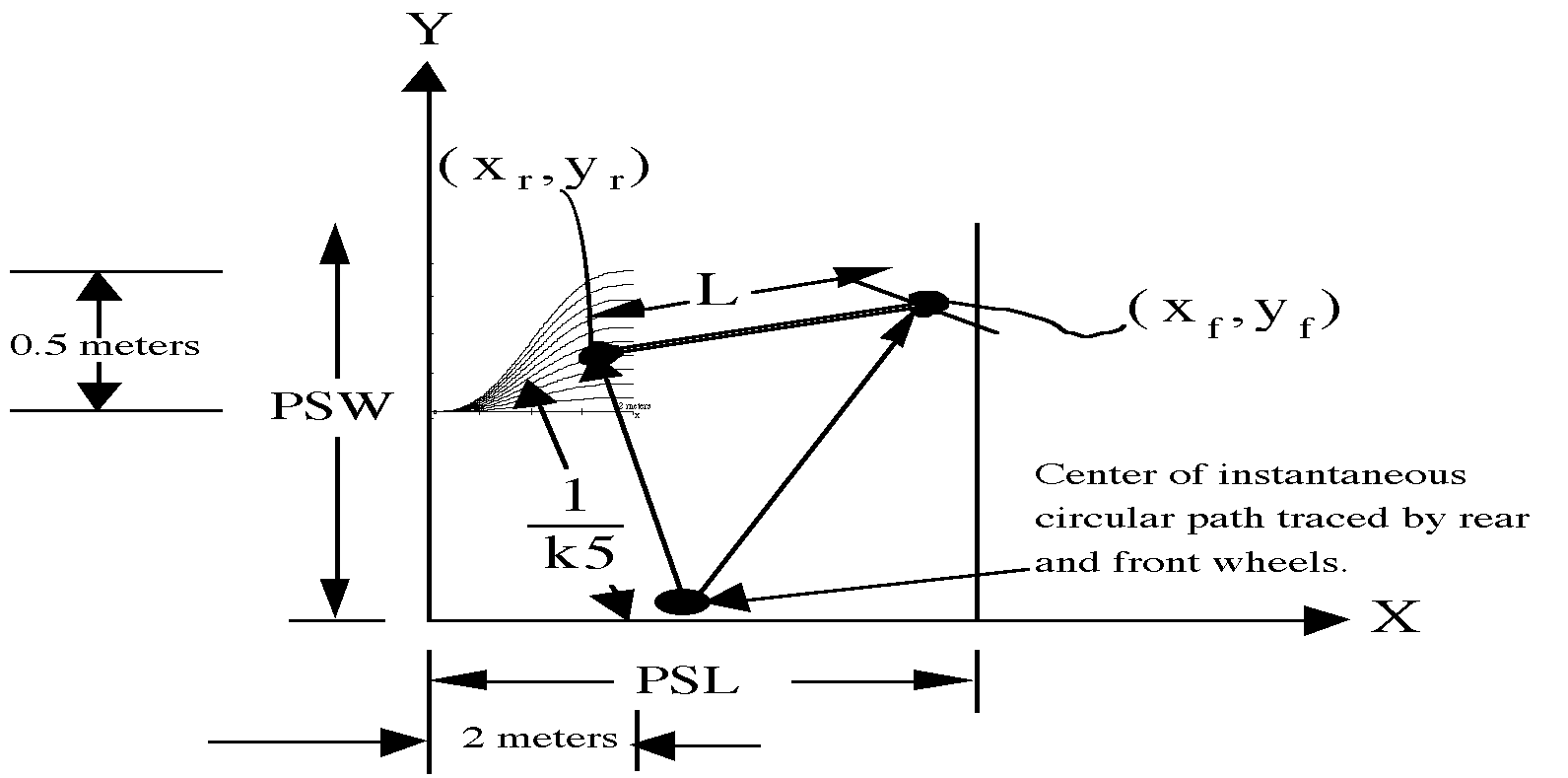
Figure 3.1-1. Parking Constraints.
The parking space has straight walls which form a "U". Some sample maneuvers are shown.
The car must avoid collision with the walls of the parking space (i.e., the car in front and the car in back) and fit into the parking space. The rear-path curvature must be strictly less than the maximum-allowable curvature (|k5|<kmax)7. The rear path has specified slope and curvature at the maneuver end-points.
Initially we investigated several s-shaped curves (two circular arcs, a cosine curve, and a fifth-order polynomial) to determine their geometric suitability for representing the path traced in parking a car. It was shown that while all of them can accommodate initial and final position and orientation constraints, only the fifth-order polynomial accommodates initial and final curvature. The simpler curves have the advantage of allowing the path to be traversed (assuming constant acceleration and deceleration) about as rapidly as the fifth-order polynomial and achieve greater penetration into the parking space. The disadvantage of these curves is that they incur an additional time penalty in straightening out the wheels at the maneuver end-points. This study showed representative examples of the curves and illustrated the effect of the turning radius of the car on the time required to park it [Lyon 1990].
The rear path during a single maneuver is represented as a (single-valued) function yr = f(xr). The general form of a fifth-order polynomial is
 (3.1)
(3.1)
 (3.2).
Let the car be parallel with the curb at the maneuver end-points:
 (3.3).
It is also desirable to have the front wheel of the car parallel to the curb at
the maneuver end-points. This will save steering-wheel alignment time at the
beginning and end of the maneuver. Steering while the car is in motion also
reduces tire wear. The wheels are parallel to the curb when the rear path has
zero slope and curvature. The rear-path end-points have X-coordinates zero and
PSL-L. Thus the fifth-order polynomial, as a function of the X-coordinate, must
have zero curvature at xr = 0 and
xr = xe, so that
k5(0) = k5(xe) = 0 (3.4).
Where k5=f(xr) is the curvature and 1/k5 is the instantaneous rear turning radius. The curvature is given [Faux 1979] by:
 (3.5).
To enforce the curvature end-point constraints, k5(0)=k5(xe) = 0, it is
necessary and sufficient to require that the second derivatives equal zero at
the rear-path end-points:
 (3.6)
(3.6)
As shown in Appendix A, enforcing the docking constraints (3.3 and 3.6) results in
 (3.7).
Substituting (3.7) into (3.5) yields
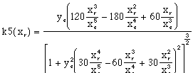 (3.8)
(3.8)
for the rear-path curvature. Recall that xe, is the target X-component of the rear path and ye is the Y-component of the amplitude of the rear path.
Since cars have a limited turning radius, an inequality constraint is imposed on the maximum curvature (kmax) of the rear path. This constraint causes the amplitude (ye) of the fifth-order polynomial to be a function of the maximum curvature. This function is computed numerically, because it requires solving the curvature equation for a maximum.
To ensure that the curvature is constrained, |k5(xr)| < kmax, we find the extrema of the curvature by setting the derivative of the curvature equal to zero and solving for xr. This yields the positions of the extrema at the inflection points used to find the maximum curvature. The extrema cannot occur at the end-points since the curvature is zero there. The non-linear nature of this problem requires a doubly-nested numerical method for finding the maximum permissible fifth-order polynomial deflection. The inside loop establishes the maximum curvature for a given deflection and the outside loop alters the deflection. Exact solutions may be found for specific cases, but analytic solutions are not forthcoming.
yr k5
 xr
xr
 xr
xr
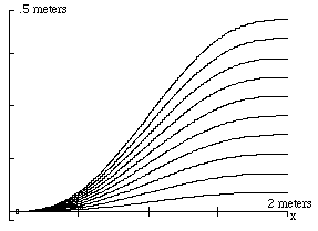
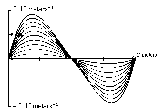
Figure 3.1.2-1. Family of Fifth-Order Polynomials and Respective Curvatures.
The curves have varying amplitude with zero slope and curvature at the maneuver end-points.
The location and value of the curvature maximum varies as a function of the amplitude. In Figure 3.1.2-1, xe = 2 meters.
There is only one fifth-order polynomial with a curvature maximum, over the feasible range of xr, equal to kmax. The maximum curvature, kmax, and the maneuver room, xe, are car and parking-space specific.
We have shown that the parking problem requires specialized docking constraints. The fifth-order polynomial is a minimum-order polynomial designed to comply with these constraints. Numeric techniques are used to find the fifth-order polynomial with curvature limited by the turning radius of the car.
Further constraints to be addressed include limits on 1-D and steering acceleration.
Nonholonomic-dynamical systems arise whenever there are non-integrable relations between coordinates and their time derivatives [Fox 1987] and these systems must be solved numerically [Latombe et al. 1989]. This is not surprising, considering the non-linear nature of the coupled differential equations. With nonholonomic constraints, you can go anywhere, but not any way!
The word "nonholonomic" comes from the Greek and means "not altogether lawful." Suppose that us is the sth state variable of a system with N state variables, then a constraint not reducible to the form

is a nonholonomic constraint. Examples of nonholonomic constraints include inequality constraints (i.e., the car must be contained within the parking space). In fact, any dynamical system of two of more particles is subject to at least one nonholonomic constraint.
If a system of L independent equations of constraint of the form
 (3.9)
(3.9)
does not possess L integrals of the form
 (3.10)
then the system of constraints is nonholonomic [Rosenberg 1977].
An important characteristic of the nonholonomic constraints is that the dimension of the space of accessible configurations is not reduced by nonholonomic constraints. Therefore, given the proper set of maneuvers, one may drive to any prescribed configuration.
In summary, a system is nonholonomic when the equations of constraint cannot be integrated. A characteristic of a nonholonomic system is that the number of parameters exceeds the number of degrees of freedom. The excess is equal to the number of non-integrable equations of constraint [Korenev 1967].
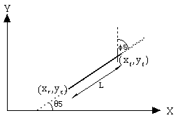
Figure 3.2.1-1. 2-D Car States.
Car orientation ([[theta]]5) and steering-wheel angle ([[phi]]5) are in radians. The front of the car (xf,yf) and length (L) are measured in meters. Width is neglected. The car length and orientation are used to compute the car-rear location, for reverse maneuvers.
The angle, [[theta]]5, the car makes with the X-axis is called the car orientation. The angle of the front wheel with respect to the main axis of the car, [[phi]]5, is called the steering-wheel angle. The distance traversed by the front wheel is denoted s5. The kinematic equations of car motion are derived by Barraquand and Latombe and nonholonomically constrain the car [Latombe et al. 1989]. The nonholonomic nature of the constraints is evident in equations (3.11) through (3.13):
 (3.11)
 (3.12)
 (3.13).
Equations (3.11) and (3.12) arise because the point at which the wheels touch the ground has zero velocity with respect to the car (the no-slip condition)[8]. The no-slip condition requires car travel in the direction of its wheels. The steering-wheel angle, [[phi]]5, is measured relative to the car orientation. The velocity of the front of the car is tangent to the front wheel. Dividing (3.12) by (3.11) results in
 (3.14).
Proof of equation (3.13):
The front of the car turns about a circle whose radius, r, is measured by the perpendicular distance between the front wheel and a ray fired from the rear axle of the car as shown in Figure 3.2.1-2.
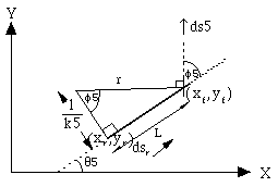
Figure 3.2.1-2. The Turning Radius of the Car.
The turning radius of the car is measured by the perpendicular distance between a ray emanating from the rear axle of the car and front wheel.
By applying trigonometric relations to Figure 3.2.1-2, and the result (from differential geometry) that the derivative of the arc length of any path with respect to the angle of the ray to the path is equal to the radius of curvature, we obtain (3.13) Q.E.D.
Since the rear wheel is always parallel with the car axis,
 (3.15)
results.
The rear of the car is fixed relative to the front of the car and this results in
 (3.16).
For the rear path to track a curve whose curvature is k5, subject to constraints (3.11), (3.12) and (3.13), we must set the steering-wheel angle so that
 (3.17).
Given constant steering angle, the front and rear of the car trace the arc of a circle, and orientation changes as a linear function of s5 [Barraquand et al. 1989].
Figure 3.2.2-1 shows the numerical solution and the tracks of the center of the front and rear of the car as a function of the path length of the front of the car.
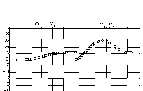
Figure 3.2.2-1. Example Maneuver
All units are in meters. We show the solution to the nonholonomically constrained initial-value problem.
Figure 3.2.2-2 shows that the car orientation and curvature are zero at the maneuver end-points, and this means that the car is parallel with the curb and that the front wheel is straight.
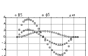
Figure 3.2.2-2. Example Angles and Curvature
The steering-wheel angle, car orientation and curvature are zero at the maneuver end-points. the curvature for the rear of the car as described by the fifth-order polynomial (k5) is in meters -1.The steering-wheel angle and car orientation are in radians.
Tabulated results show that the maximum curvature is 0.223 meters-1, the Y-component of the final rear deflection is 0.23 meters and that the maximum steering-wheel angle is 0.526 radians. Thus, the state variables which describe the car motion are feasible.
Several experiments were performed to measure the maximum Y-deflection for various values of PSL-L. The maximum Y-deflection is the peak lateral excursion required for a maneuver. A graphical summary and quadratic approximation to the data is shown in Figure 3.2.2-3.
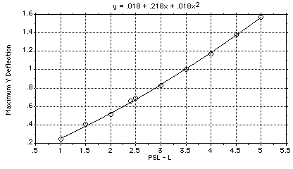
Figure 3.2.2-3. Maximum Y-Deflection vs. PSL-L.
Several experiments show that the maximum Y-deflection is almost quadratic in PSL-L. When the maximum Y-deflection exceeds the available lateral maneuver room, the car will mount the curb.
If the car approaches the curb, the parking space width cannot be considered infinite and the car must back in to the space. If the car were to pull forward, without sufficient space between the car and the curb, the car would mount the curb.
Several experiments were performed to measure the Y-deflection at the maneuver end-points for various values of PSL-L. A graphical summary and a quadratic approximation to the data is shown in Figure 3.2.2-4. The deflection into the parking space is a quadratic function of the available maneuver room. Simple circular arcs also yield a quadratic deflection as a function of PSL-L.
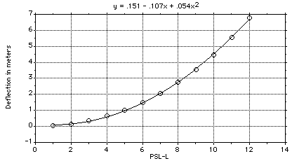
Figure 3.2.2-4. Y-Deflection vs. PSL-L.
Several experiment show that the deflection of the car at the maneuver end-points is almost quadratic in PSL-L.
This chapter established the state variables which determine car configuration as a function of front-wheel path-length. In subsequent chapters, path-length will be a function of time, and the spatial differential equations given here will be used in their temporal form.
Open-loop control establishes upper and lower bounds on controller performance by modeling an observer with and without plant-model error. This chapter reports performance bounds on plant-model overshoot when there is acceleration error.
Let us establish the control nomenclature used in this thesis. Figure 4-1 shows an overview of an open-loop system with three main parts: the controller, observer and plant. We assume that the plant model may incorporate error.
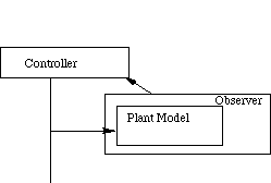
Figure 4-1. Open-loop Control.
The observer uses controller-input to estimate plant states. The controller uses the plant-state estimate to formulate input.
The controller uses the plant-state estimation produced by the observer to determine the control signals. These signals are applied to the plant model and the plant. Error in the plant model will cause a reaction to the control signals which is different from the plant's reaction. This is called open-loop control because there are no sensors between the plant and the observer. The observer will perform sensor fusion to update the plant model in the closed-loop control regime of Chapter 5. The difference between closed-loop and open-loop control is the presence of sensor feedback between the plant and the observer, otherwise the control regimes are identical.
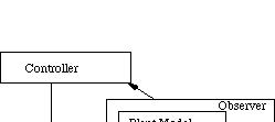
Figure 4.1.1-1. Error-Free Control.
The observer's plant model is developed in parallel with the controller to establish a test-bed for constructive modeling.
The controller issues 1-D acceleration commands which the plant model follows, without error. To simplify simulation, we assume that reverse torque is used to brake the car and to cause backward motion. Electric cars permit the application of reverse torque during a forward maneuver.
Parking space walls are static constraints and are considered known a priori. The literature survey in Chapter 2 established the minimum parking space length as 4.6 meters and the maximum parking space length as 6.7 meters. Further, it was established that the smallest cars are 4.3 meters long. We assume that the parking space is 6.7 meters long and that the car is 4.3 meters in length (3.88 meters axle to axle). As a result, the maximum distance from the front of the car to the opposite wall of the parking space (i.e., the next car) is 6.7 meters - 4.3 meters = 2.4 meters. Therefore, the largest displacement during any single maneuver is 2.4 meters, the value used for simulation.
The distance required to stop a car moving at speed f(ds,dt) is given by:
 (4.1)
(4.1)
where
db is the distance needed to stop the car,
f(ds,dt) is the speed, and
asmin is the braking deceleration.
In this thesis, speed is a scalar quantity which can go negative. During a reverse maneuver, speed is negative, and watching the integral of the speed is like watching an odometer which turns backward when in reverse. This has advantages which will become evident in simulation.
Little information is available on average acceleration and deceleration for a car over the 0 to 2.4 meter range. For a comfortable ride, the vehicle acceleration must be less than 1.95 m/s2 [Hauksdottir and Fenton 1985]. Power-train models show that car acceleration is highly non-linear and not constant in the first 2.5 seconds of operation [Ha et al. 1989].
Due to the lack of car acceleration studies in the 2.4 meter range and because car simulations may be verified with a real car, field tests were performed. Two experiments with three trials each established estimates for rates of acceleration and deceleration. The test vehicle was a 1989 Chevy Blazer truck. Experiments showed that the test vehicle accelerates at 0.83 m/s2 and decelerates at 1.4 m/s2 in a 2.4 meter interval.
When car position, s, plus braking distance, db, exceeds the objective path length for the car (2.4 meters), the brakes are applied. In the forward maneuver, the acceleration command is given by the following expression:
 (4.2).
Integration of the speed results in path length. The initial path length and speed are equal to zero.

Figure 4.1.2-1. Graph of 1-D Motion.
Position is in meters, speed is in meters per second and acceleration is in meters per second squared.
The resting position of the car is 2.41 meters, an overshoot of 0.01 meters ( a 0.4% error). The STELLA step size (dt) is 0.01 seconds, and this causes the overshoot. For example, the identical simulation with a STELLA step size of 0.1 seconds results in a resting position at 2.61 meters, an overshoot of 0.2 meters (8% error). Step sizes of smaller than 0.01 seconds lead to large simulation times.
Note that the peak speed of 1.59 m/s (3.6 mph) and the total simulation interval of three seconds are consistent with field tests. In addition, 1.59 m/s is slow enough so that a limit on the speed, i.e., a coasting period, is unneeded.
In summary, no acceleration error and dt=0.01 seconds caused a 0.4% overshoot. This is due to temporal quantization, since the same model with dt=0.1 seconds resulted in an 8% overshoot.
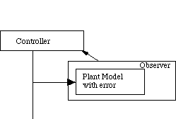
Figure 4.1.3-1. Open-loop Control using a Plant Model with Error.
The observer uses controller input to estimate plant states. The controller uses the plant-state estimate to formulate input.
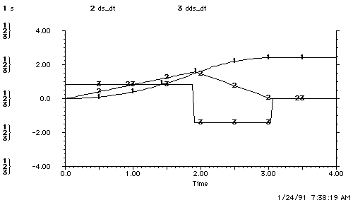
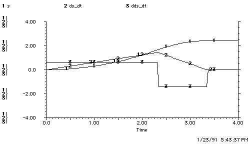
The 25% underestimation of acceleration could result from a combination of payload and terrain changes which are unpredictable, i.e. hills, cargo, snow or rolling resistance. Overestimating acceleration or underestimating deceleration is a non-catastrophic failure, since it results in undershoot. The opposite error can cause a collision, and this is a catastrophic failure. We investigate separately the effects of underestimating acceleration and overestimating deceleration, then combine the errors for a worst-case scenario. Equation (4.3) shows a 25% overestimation of the acceleration of the plant model in the observer.
 (4.3)
(4.3)
Where
 = acceleration of the plant.
 = linear acceleration command used by the plant-model.
The acceleration error causes the plant's maneuver to take longer than the
observer's. A comparison of the overshoot indicates that the acceleration error
makes no difference. From the observer's point of view, the plant stopped at
2.41 meters in both simulations. As would be expected, however, the plant
overshot by 1.16 meters (see
Figure 4.1.3-2b).
In summary, the observer's plant model has a 25% lower acceleration than the car. The observer uses the plant model as a reference and so is applying the gas when it is actually time to brake. The result is that the car overshoots.
Now assume there is error only in the estimate of the deceleration,
 (4.4)
(4.4)
and the braking distance, as computed by the observer, is updated to:
 (4.5).
Figure 4.1.3-3b shows early halting caused by the observer's overestimate of the plant deceleration. The effect on the plant is shown in Figure 4.1.3-3c.
Figure 4.1.3-3 shows that the observer's overestimation of the plant's ability to brake causes the brakes to be applied too late to stop in the allotted space. The plant reaches the same peak speed as the observer because there is error in deceleration only. The deceleration overestimation results in overshoot and an increased maneuver time.
Overestimation of deceleration leads to a plant travel of 2.66 meters, or a 0.26 meter overshoot.
We now combine the effects of a 25% acceleration and a deceleration error into a single simulation. The combination of the errors is obtained by changing the control law in (4.4) to:
 (4.6).
The observer reacts as expected, having a long period of acceleration with an abbreviated deceleration. This is shown in Figure 4.1.3-4b.
Figure 4.1.3-4 shows that the observer's overestimation of the plant's ability to brake and underestimation of the plant's ability to accelerate compounds the problem.
The resting position of the plant is 3.84 meters. The objective position is 2.40 meters, and the difference is 1.44 meters, a 60% overshoot. In the following figures, position is in meters, speed is in meters per second and acceleration is in meters per second squared.
a. The Error-Free Plant
b. The Observer's Plant Model
c. Open-Loop Control of the Plant
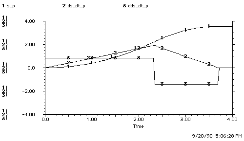
Figure 4.1.3-2. Underestimation of Acceleration.
Figure b shows the plant-model with 25% underestimation of acceleration. Figure c shows the observer's underestimation of acceleration leading to overshoot. The observer underestimates the plant's ability to accelerate and so accelerates for too long. The plant reaches a higher peak speed and therefore takes longer to slow down and maneuver time increases.
a. The Error-Free Plant

b. The Observer's Plant Model
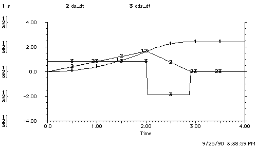
c. Open-Loop Control of the Plant
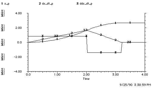
Figure 4.1.3-3. Overestimation of Deceleration.
Figure a shows observer overestimation of the plant's deceleration and this causes early halting. Figure c shows overestimation of plant deceleration by the observer causing overshoot.
a. The Error-Free Plant

b. The Observer's Plant Model
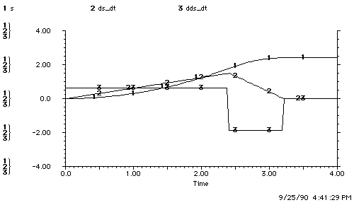
c. Open-Loop Control of the Plant

Figure 4.1.3-4. Underestimation of Acceleration and Overestimation of Deceleration.
Figure b shows the observer estimates with 25% acceleration and deceleration error. Figure c shows the objective position (2.4 meters) being overshot by 60%.

Figure 4.1.3-5. Summary of Open-loop Errors.
The overshoot from the combined errors almost linearly sums to form the combined overshoot. The objective position is 2.41 meters.
Figure 4.1.3-5 shows that a 25% underestimation of acceleration causes a 48% overshoot and that a 25% deceleration error causes a 10.8% overshoot. It also shows that the combined acceleration and deceleration errors causes a 60% overshoot.
Given the errors in the plant model, the overshoot can be reduced (but not eliminated) only through sensor feedback. The sensor feedback reduces overshoot because it improves the observer's braking-distance estimate and this leads to earlier braking by the controller. Even perfect plant-state estimates won't eliminate overshoot because the braking-distance estimate is a function of the overestimated deceleration.
In addition to considering acceleration and deceleration error we consider rolling resistance as a source of error. Appendix C examines drag as a source of error in modeling the plant and shows that rolling resistance takes only 1% of the engine's power and is therefore negligible.
This section uses a temporal nonholonomic system of differential equations which are derived from the spatial nonholonomic system of differential equations in Chapter 3. To reflect the change of the independent variable from the X-component of the rear of the plant (xr) to time (t), and to make explicit that these equations are for the plant model, we introduce the following notation:
x [[equivalence]] X-component of the front of the plant model,
y [[equivalence]] Y-component of the front of the plant model,
f(dx,dt) [[equivalence]] rate of change of the X-component of the front of the plant model,
f(dy,dt) [[equivalence]] rate of change of the Y-component of the front of the plant model,
s [[equivalence]] length of the path traveled by the plant-model,
sdo13(
 )front-wheel plant-model speed,
[[theta]] [[equivalence]] plant-model orientation, angle formed by the main axis of the plant with the X-axis of a Cartesian coordinate frame aligned with the curb,
f(d[[theta]],dt) [[equivalence]] rate of change of the plant-model orientation,
[[phi]] [[equivalence]] steering-wheel angle relative to the longitudinal centerline of the plant model and
f(d[[phi]],dt) [[equivalence]] rate of change of the steering-wheel angle of the plant model relative its longitudinal centerline.
To obtain the temporal differential equations from the spatial differential equations shown in (3.11-3.13), multiply both sides of equations (3.11-3.13) by the time-variant speed, f(ds,dt) , and substitute the plant-model notation for the fifth-order polynomial notation, to obtain:
 (4.7)
(4.7)
 (4.8)
(4.8)
 (4.9).
The car pose (x, y, [[theta]]) and steering-wheel angle ([[phi]]) are shown in Figure 3.2.1-1 as static curves. The only difference is that (4.7-4.9) describe dynamic and not static curves.
In addition to the nonholonomic constraints, the rate at which the steering wheel may be turned (the second derivative with respect to time of 3.17) is limited by the rotational inertia of the steering system and the limits on steering torque.
Recall that the reference curvature in (3.8) is a function of xr. This, in turn, is a function of xf and [[theta]]5 as given in (3.16). The equations of (3.16) are valid for the plant model as well, all that remains is that x, y and [[theta]] be substituted for xf, yf and [[theta]]5. These state-variables are subject to the nonholonomic constraints of (4.7-4.9). These constraints will produce values for x and [[theta]] when the 1-D control starts the car motion. In equations (3.3) and (3.8), xe and ye are restricted by the curvature maximum and are computed before a maneuver is begun. The fifth-order polynomial traces a reference path whose curvature is tracked during a maneuver.
Since the car is subject to some overshoot we must restrict the range on the X-component of the rear of the car's deflection so that
 (4.10)
for going forward and
 (4.11)
for going backward.
All that remains is the formulation of the angular acceleration control. The steering curvature as computed by (3.8) is
 (4.12)
for going forward and
 (4.13)
for going backward. Recall that L is the length of the car, xe, the target X-component of the back of the car and ye the total deflection of the ideal fifth-order polynomial. The functional notation is omitted for brevity here. Curvature is a function of the rear-component of the X-coordinate of the car. The relationship between the front and rear coordinates is given in equation (3.16). Both are subject to the temporal nonholonomic constraints in (4.7-4.9).
The difference between this controller and the 1-D controller of Section 4.1 is the difference between a servo controller and a tracking controller [Athens and Falb 1966]. In a servo controller the command input (the objective_position) is time-invariant. In the tracking controller the command input (the reference path's curvature) is time-variant.
The control law of this open-loop 2-D nonholonomically constrained system is given by
 (4.14)
where
 (4.15).
The key decision variable is e and this is the result of a proportional plus derivative control. The control is based on the steering-wheel angle and the car orientation and this is given by
 (4.16)
where
 (4.17),
 (4.18),
and
 (4.19).
The variable, backup_lights, is set equal to one when the car is backing up. The mix ratio between the proportional and derivative control must be found by experiment. The values
 (4.20)
gave good results (See Appendix. E).
The steering-wheel angle of the car, as given by the fifth-order polynomial, makes use of the fifth-order polynomial prescribed curvature (4.12) and (4.13) and is:
 (4.21).
Implicit in the nonholonomic constraints is the dependence of car orientation on the speed of the car:
 (4.22).
The proportional component of the orientation control is obtained by numerical integration of (4.22).
The 1-D component is altered for the purpose of accomplishing multiple maneuvers. The maximum deflection of the fifth-order polynomial is limited in order to limit the curvature extrema, as pointed out in Chapter 3.
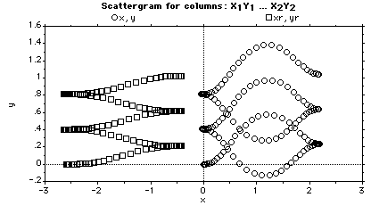
Figure 4.2.2-1. Error-Free Curvature Tracking.
An error-free plant model is used to control the plant curvature. On the left is the path traced by the rear wheel; on the right, that of the front wheel.
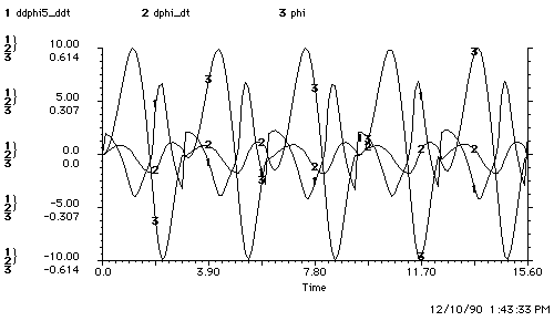
Figure 4.2.2-2. Angular Acceleration.
The resulting steering acceleration is proportional to the linear acceleration. If the plant slows down we do not need to steer as fast.
Figure 4.2.2-2 shows the maximum acceleration is 6.85 rads/s2, and the minimum is -4.20 rad/s2. The reason why the maximum and minimum steering accelerations differ is that the car is first maneuvering forward and then backward. During the backward maneuver the car is subjected to rear-wheel steering and rear-wheel steering response differs significantly from front-wheel steering response [Whitehead 1990]. An acceleration of one radian per second squared is not realistic from the driver's perspective, but with the proper gear ratios and over small angular displacement, such angular accelerations are possible.
This section on 2-D motion follows the development of 1-D motion in Section 4.1 as closely as possible. Significant deviations from the development of Section 4.1 include the symmetric-acceleration assumption and the tracking nature of the servo. It was found from experiment that the required angular acceleration exceeds the driver's ability by a factor of 18 and that the steering system must be geared up appropriately for computer control.
A 25% angular-acceleration and underestimation of the engine torque are implemented by
 (4.23)
 (4.24)
and
 (4.25).
A simulation which uses this control law gives the results shown in Figure 4.2.3-1.
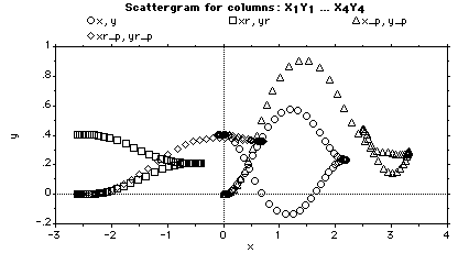
Figure 4.2.3-1. Open-Loop Control with 25% Underestimation.
The plant model in the observer is shown by the (x, y) trace. The plant is shown by the (x_p, y_p) trace.
Figure 4.2.3-1 shows the results after two maneuvers. After two maneuvers the plant state vs. the observer estimates are off by 2.5 meters in the X-component, 0.04 meters in the Y-component, 0.01 radians in the car orientation and 0.006 radians in the steering-wheel angle.
Correction is clearly needed since the errors will increase with the number of maneuvers.
In 2-D open-loop control we found that the rate at which the car approaches the curb is 0.406 m/6.0 s = 0.067 m/s for the error-free maneuvers and 0.443 m/6.0 s = 0.073 m/s for the maneuvers with error. The increase is due to the observer's underestimation of acceleration. The resting X-coordinate error after two maneuvers is 2.5 meters; this indicates the need for sensor feedback.
Section 5.1 provides an overview of the closed-loop system. Section 5.2 covers internal and external sensors with a justification for sensors whose reliability is inversely related to availability. Section 5.3 summarizes closed-loop bang-bang control for 1-D motion using internal and external sensors. Section 5.3 also shows that the 1-D sensor fusion techniques are applicable to 2-D motion and give similar improvements in plant-state estimates and controller performance.
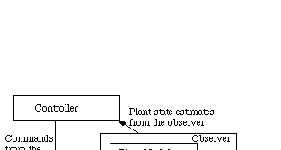
Figure 5.1-1. Closed-loop Control.
The observer uses the plant model driven by the controller commands to estimate plant states. The controller uses the plant-state estimates to generate commands. Sensor feedback is used to correct the observer's estimate of the plant states.
The observer uses a plant model and sensor measurements to estimate the state of the plant. The process that the observer uses to incorporate measurements from different sensors is called sensor fusion.
There are two classes of sensors, internal and external. Their reliability is inversely related to their availability. External sensors are more accurate than internal sensors and dominate the internal sensors when they are available.
Internal sensors measure the plant state relative to itself. An odometer is an example of an internal sensor which measures the distance a car travels by measuring tire motion. Since tires slip, the odometer will have some error. We also assume that internal sensors have a 20 hertz sampling rate. Candidate internal sensors are: the accelerometer, the tachometer and the odometer. These sensors give equivalent data. Equivalent data means that data provided by any one of the sensors may be transformed into data provided by any of the others.
External sensors measure the plant state relative to the environment. A Sonar sensor is an example of an external sensor. We assume that external sensors have a 5 hertz sampling rate.
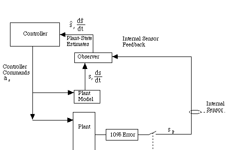
Figure 5.2.1-1. Internal Sensor Feedback.
The observer resets the plant-model's position at a rate of 20 Hertz. The observer's speed estimate is reset using consecutive pairs of position measurements.
When the switch in Figure 5.2.1-1 is closed, the observer updates the plant-model position. The odometer measures the plant position, with error. The observer also updates its estimate of the plant's speed. The speed is estimated by dividing the difference between consecutive position measurements by the sampling interval.
External sensors are assumed to be error free. During the time that external sensors are not available, the last externally sensed data is used in combination with the internal sensor to perform dead reckoning. When the external sensor is available, its data dominates the internal sensor's data, as described below.
This brings up an important point concerning error assumptions. We have tried to relax most assumptions made about sensors. For example, we do not assume that there is Gaussian noise on the sensor, nor do we assume that there will be systematic acceleration error. In fact, error could come from ice, terrain, load or any of a slew of other sources. The less we know about the errors we will encounter, the more intelligent our interpretation of sensor data must be.
Another point concerning the approach taken here is that the sensors we have selected do not provide the same data at the same rate. This avoids sensor redundancy and places emphasis on a few good sensors rather than on several lower-performance ones. In addition, the sensor dissimilarity avoids the statistical approach to sensor fusion [Pons 1989]. A new technique is developed for performing sensor fusion using sensors with widely different characteristics.
The remainder of this section describes an experiment which fuses data from 20-hertz internal sensors with 10% error and 5-hertz external sensors with no error. This data is available to the observer. The only external sensor is the sonar, and the only internal sensor is the odometer. The odometer data is fused with the sonar data, and the resulting estimate is used to correct the plant-model which overestimates acceleration by 25% and underestimates deceleration by 25%.
Figure 5.2.3-1 shows a block diagram of the internal sensor and external sensors used by the observer.
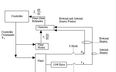
Figure 5.2.3-1. Internal and External Sensors.
A five-hertz switch is used to symbolize the limitation of the sampling rate for the external sensor.
We assume that the car moves in 1-D and so the X-component of the front of the plant, and the length of the path traveled by the plant front-wheel, are identical. This is also true for the plant model. The results of this simulation are shown in Section 5.2.4.
Figure 5.2.4-1 shows a comparison of 1-D control regimes. Several plant states and observer estimates are shown. The observer estimates show that the controller is performing optimally, given the observer's information. As the information to the observer improves, so does its plant-state estimate and the resulting controller performance.
The overshoot of the plant when it halts is a useful criterion. Better observer estimates will reduce this overshoot. The overshoot is 3.76 m - 2.41 m =1.35 m for the open-loop case. The only action performed by the controller is the application of the brakes at the right moment. The data for the open-loop control is presented graphically in Figure 4.1.3-5. Both acceleration underestimation and deceleration overestimation were used for the open-loop results, since these assumptions maximized the overshoot.
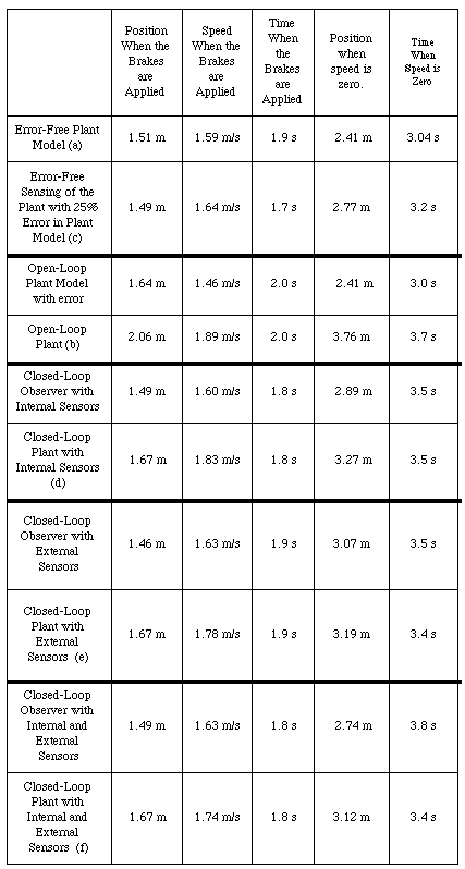
Figure 5.2.4-1. Comparison of 1-D Control Regimes.
The 1-D error-free sensing of the plant with 25% error in the plant model sets a best-case performance bound for closed-loop control with 0.36 m overshoot. The open-loop plant shows the worst-case response, with 1.35 m overshoot. The 1-D closed-loop plant with internal sensors has a 0.86 m overshoot. The 1-D closed-loop plant with external sensors has a 0.78 m overshoot. The 1-D closed-loop plant with internal and external sensors has 0.71 m overshoot. The letters in parenthesis refer to figures.
The 1-D error-free plant model was discussed in Section 4.1.1. The 1-D error-free plant model provides a best-case bound on the controller's performance. The position of the 1-D error-free plant model, and of the plant model with error under open-loop control, is 2.41 meters, when the speed is zero. This shows that the controller is performing optimally given the observer's information.
The 1-D error-free sensing of the plant, with 25% error in the plant model, sets a lower best-case performance bound for closed-loop control. Sensors are error-free and running at the simulator rate of 100 hertz. Without using an adaptive reference model, and with no prior knowledge of the plant-model error, this must be the best performance that we can expect from any sensor fusion scheme. The overshoot using this scheme is 2.77 m - 2.41 m = 0.36 m.
The 1-D closed-loop plant with internal sensors has 25% error in the plant-model and 10% error in the internal sensors. The internal sensors are sampled at 20 hertz (Figure 5.2.1-1). The overshoot of the plant position when the speed is zero is 3.27 m - 2.41 m = 0.86 m.
The 1-D closed-loop plant with external sensors has 25% error in the plant-model and no error in the external sensors. Also, the external sensors are sampled at 5 hertz. The overshoot of the plant position when the speed is zero is 3.19 m - 2.41 m = 0.78 m.
The 1-D closed-loop plant with internal and external sensors has 25% error in the plant-model. There is no error in the external sensors. There is 10% error in the internal sensors which are sampled at 20 hertz (Figure 5.2.3-1). The overshoot of the plant position when the speed is zero is 3.12 m - 2.41 m = 0.71 m.
In the 1-D closed-loop plant with internal and external sensors, the performance after a single maneuver is slightly better than using external sensors alone. An examination of the position of the plant when the speed is zero shows that the fusion of external sensors with internal sensors will reduce overshoot by 0.07 meters, for a single maneuver. It is also seen that internal sensors reduce the single-maneuver overshoot obtained from open-loop control by 1.35 meters - 0.89 meters = 0.46 meters. Closed-loop sensor fusion reduce single-maneuver overshoot by 0.64 meters over the open-loop case.
The observer underestimates the acceleration and overestimates plant's ability to brake. The result is that the plant accelerates for too long and decelerates for too short a time. The underestimation of acceleration in the plant model causes the plant to attain a higher speed than the plant model. At higher speeds it takes longer to brake, even when the deceleration is known accurately.
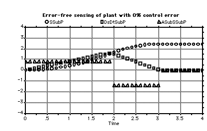
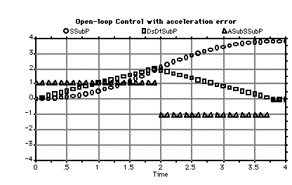
a.) Error-free sensing of plant b.) Open loop
with error-free plant model
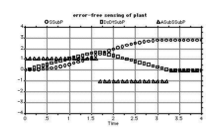
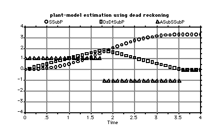
c.) Error-Free Sensing of the Plant d.) Internal Sensors
with 25% Error in Plant Model
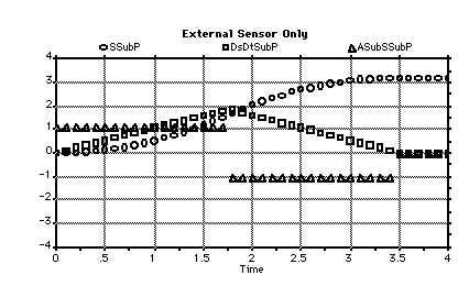
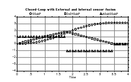
e.) External Sensors f.) Sensor Fusion
Figure 5.2.4-2. A Single Maneuver and 1-D Control Regimes.
The above graphs show the length of the path traveled by the plant front-wheel (SSubP), the front-wheel plant speed (DsDtSubP) and the 1-D acceleration for the plant (ASubSSubP).
Figure 5.2.4-2 shows several 1-D control regimes running in simulation over a four second interval. Figure 5.2.4-2a shows an upper-bound on parking performance. This can never be attained when the reference model has error. Figure 5.2.4-2c shows the result of error-free sensors sampling at the simulator clock rate (100 hertz) using an erroneous reference model. Figure 5.2.4-2b shows open-loop control (the limiting case as sensor sampling rates approach 0 hertz).
The sensor fusion technique used here is used in the next section on 2-D motion and yields similar results.
As in Chapter 4, this section summarizes a study of 2-D control using the fifth-order polynomial to generate a reference path. Bang-bang control is used to adjust the acceleration and the steering-wheel angle of the car. Nonholonomic constraints are used by the observer to compute pose (position and orientation).
We compare open-loop control against several closed-loop control regimes. These regimes differ in the sensor data provided to the observer. Open-loop control is based on a plant-model with error and does not use sensors. The closed-loop control regimes are based on internal sensors (dead reckoning), external sensors and a combination of both. As a basis for comparison we also show control based on error-free sensing of the plant states. This provides a best-case limit on the parking performance and can be compared with open-loop control (which provides a worst-case limit on parking performance).
External sensors are sampled without error at 5 hertz and internal sensors are sampled with 10% error at 20 hertz. The plant-model is used between sensor readings and is always available to the controller. The plant-model has 25% steering and linear acceleration error. Sensors compensate for the error in the plant-model, improving performance.
The ideal steering-wheel angle is a function of the fifth-order polynomial's curvature (as shown in Chapter 4). The controller is not able to set the plant's steering-wheel angle except by banging on the steering system. The control law described in Chapter 4 is not altered. The only change is in the accuracy of the plant-state estimate given to the controller by the observer.
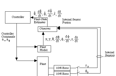
Figure 5.3.1-1. Dead Reckoning.
Dead reckoning uses only the internal sensors to obtain a better estimate of the plant-states. As in Figure 5.2.1-1, the internal sensors are fast and error-prone. The only difference is the additional sensor for the steering-wheel angle, [[phi]]p.
The sample-and-hold switches for the odometer and the steering-wheel angle meter are actuated simultaneously and at 20 hertz. There is a single simulator delay interval needed before the sample-and-hold attains the measured value. The values measured by the internal sensors are multiplied by 0.90 to model the 10% internal sensor measurement error.
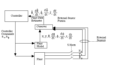
Figure 5.3.2-1. External Sensors in 2-D.
The 2-D external sensors are able to read the pose (position and orientation) of the car with respect to its environment. This gives the observer an error-free measure of the car's pose at a rate of five hertz.
It will be shown that control with external sensors is not much better than control with internal sensors and that control with both internal and external sensors is better than control with either one alone.
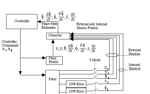
Figure 5.3.3-1. Internal and External Sensors Used by the Observer.
Internal sensors are sampled at 20 hertz and have 10% error while external sensors are sampled at 5 hertz and have no error.
The plant model has a 25% error in linear and steering acceleration. The observer fuses the internal and external sensors to reduce the plant-model error. The plant steering-wheel angle is measured directly at 20 hertz with 10% error. This is used to improve the observer's estimate of the steering-wheel angle. External sensors cannot help improve the observer's estimation of the steering-wheel angle because the change in the plant's pose lags behind the change in the steering-wheel angle. Car orientation is directly measured by an external sensor, without error, and is used to update the observer's estimate.
During the intervals of time when the externally sensed plant orientation is not available, the observer uses the nonholonomic constraints on orientation to incorporate the internally sensed estimate of the steering-wheel angle with the fused estimate of speed. Thus
 (5.1)
(5.1)
is the rate of change of orientation computed by fusing information from internal sensors. Orientation is obtain via numeric integration of (5.1) and exhibits cumulative error which is corrected by the external orientation sensor. This is shown in Figure 5.3.3-2.

Figure 5.3.3-2. The Observer's use of the External Orientation Sensor.
The plant's orientation (ThetaSubP) is sampled accurately at 5 hertz by the orientation sensor whose output is denoted ThetaSubP5. In between sensor samples the observer uses (5.1) to compute an estimate of the plant's orientation (ThetaHat).
Similarly, reference orientation is computed using
 (5.2).
Finally, the difference signals used to compute when to bang on the steering combine (5.1) and (5.2) to obtain:
 (5.3).
This is control law is just like that of Chapter 4, except for the introduction of the sensor feedback for improving the plant-state estimates.
The fused estimate of speed is the result of numerically differentiating the odometer reading at 20 hertz to obtain a tachometer reading with error, adjusted by the derivative of the positional change using the external sensors. The observer's estimate of the speed of the plant diverges from the true value of the plant. Since the odometer has 10% error it follows that the minimum error in the derivative of the odometery is 10% In addition, we cannot account for what the car path looks like in between sensor samples. This is particularly important in the case of the 5 hertz external sensor which actually harm the observer's estimate of the plant's speed at low velocity. This is shown in Figure 5.3.3-3.

Figure 5.3.3-3. The Observer's Estimate of Speed.
DsDt is the speed of the plant model. ApproxDsDtP20 is the 20 hertz derivative of the odometer. ApproxDsDtP5 is the 5 hertz derivative of the external sensors. DsDtHat is the observer's estimate of the plant's speed. DsDtSubP is the speed of the plant.
The external sensors are too slow to help estimate the arc-length of the path along the maneuver, and so the plant-model arc-length is updated directly by the odometer at 20 hertz with 10% error. This shown in Figure 5.3.3-4.

Figure 5.3.3-4. The Observer's Estimate of Path length.
The plant's front-wheel path length (SSubP) is sampled with 10% error at 20 hertz by the odometer whose output is denoted OdSubP20. In between sensor samples the observer uses the plant model to compute an estimate of the plant's front-wheel path length (SHat).
Figure 5.3.4-1 shows a comparison of 2-D control regimes. Since there is no single objective function to optimize, several plant states and observer estimates are shown. The observer estimates are shown in order to establish that the controller is performing optimally given the observer's information. As the information to the observer improves, so does its plant-state estimation and the resulting controller performance.
In the 2-D open-loop control with error in the plant model, we established the worst-case bound on controller performance. Open-loop control is based on a plant-model with error and does not use sensors. This was discussed in Chapter 4 where engine and steering acceleration were underestimated by 25%. The overshoot of the plant when the speed is zero is a useful criterion and is 3.76 m - 2.41 m =1.35 m. Better observer estimates will reduce this overshoot.
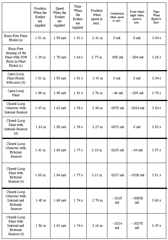
Figure 5.3.4-1. Comparison of 2-D Control Regimes.
The open-loop plant shows the worst-case response with 1.35 m overshoot. The 2-D error-free sensing of the plant, with 25% error in the plant model, sets a best-case performance bound for closed-loop control with 0.36 m overshoot. The 2-D closed-loop plant with internal sensors has a 0.86 m overshoot. The 2-D closed-loop plant with external sensors has a 0.80 m overshoot. The 2-D closed-loop plant with internal and external sensors has a 0.75 m overshoot.
The 2-D error-free sensing of the plant, with 25% error in the plant model, sets a lower best-case performance bound for closed-loop control. Sensors are error-free and running at the simulator rate of 100 hertz. Without using an adaptive reference model, and with no prior knowledge of the plant-model error, this must be the best performance that we can expect from any sensor-fusion scheme. The overshoot using this scheme is 2.77 m - 2.41 m = 0.36 m.
The 2-D closed-loop plant with internal sensors has 25% error in the plant-model and 10% error in the internal sensors. Also, the internal sensors sample at 20 hertz. The overshoot of the plant position when the speed is zero is 3.27 m - 2.41 m = 0.86 m.
The 2-D closed-loop plant with external sensors has 25% error in the plant-model and no error in the external sensors. Also, the external sensors sample at 5 hertz. The overshoot of the plant position when the speed is zero is 3.21 m - 2.41 m = 0.80 m.
The 2-D closed-loop plant with internal and external sensors has 25% error in the plant-model. There is no error in the external sensors. which sample at 5 hertz. There is 10% error in the internal sensors which sample at 20 hertz. The overshoot of the plant position when the speed is zero is 3.16 m - 2.41 m = 0.75 m.
In the 2-D closed-loop plant with internal and external sensors, the performance after a single maneuver is slightly better than using internal sensors alone. An examination of the position of the plant when the speed is zero shows that the fusion of external sensors with internal sensors will reduce overshoot by 0.11 meters, for a single maneuver. It is also seen that internal sensors reduce the single-maneuver overshoot obtained from open-loop control by 0.49 meters. Closed-loop sensor fusion reduced single-maneuver overshoot by 0.60 meters over the open-loop case. This compares with the 1-D sensor fusion which reduced the overshoot by 0.71 m (as shown in Section 5.2.4).
If the orientation is non-zero at the maneuver end-point, the controller will bang on the steering in an attempt to correct the orientation. The plant is moving slowly at the maneuver end-point and steering changes have less effect on the plant's orientation. Even if the orientation is zero, the steering-wheel of the plant never stays at zero. This is due to steering reversals after every three bangs. The three bangs last three hundredths of a second, each of which turn the front wheel by f(1,2) 50 radians/s2 x (0.03)2 = 0.0225 radians (when the steering velocity is zero at the time of the bang). This delay is due to the two integrators needed to numerically compute the steering-wheel angle from the applied steering acceleration and to the delay in the controller's decision to bang. The controller's decision to bang is delayed by a simulator time interval (0.01 seconds) because of the next-state equations used in the simulation.
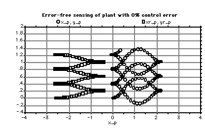
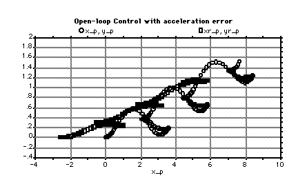
a.) Error-free sensing of plant b.) Open loop
with error-free plant model
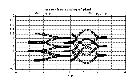
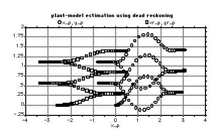
c.) Error-Free Sensing of the Plant d.) Internal Sensors
with 25% Error in Plant Model
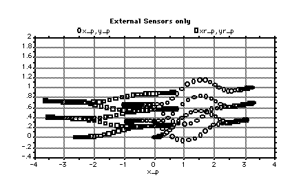
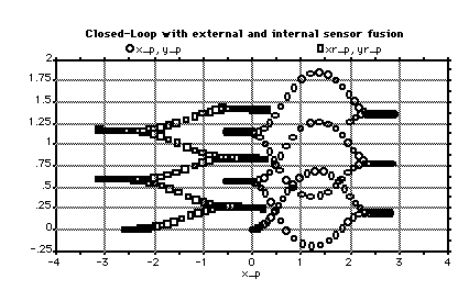
e.) External Sensors f.) Sensor Fusion
Figure 5.3.4-2. Multiple-Maneuvers and 2-D Control Regimes.
In cases show the position of the front (x_p, y_p) and rear (xr_p, yr_p) of the plant sampled at uniform time intervals. The data tends to bunch up at the maneuver end-points where the plant is moving slowly.
Figure 5.3.4-2 shows several 2-D control regimes running in simulation over a twenty second interval. Note that the open-loop control with acceleration error has so much overshoot that the scale of Figure 5.3.4-2a had to be altered. In addition, Figure 5.3.4-2a shows an upper-bound on parking performance. Figure 5.3.4-2c shows that error-free sensing does lead to a deflection smaller than the closed-loop sensor fusion show in Figure 5.3.4-2f. The reason is that the rate at which the plant proceeds along the Y-axis is a quadratic function of the available maneuver room. Since the sensor fusion case takes more room to maneuver (due to overshoot), it is able to proceed into the space faster.
In Figure 5.3.4-2a, there is no error in the plant's maneuver and so none accumulates. However, in Figure 5.3.4-2b, the error accumulates and must be reduced with sensor feedback. Either external or internal sensor feedback will keep the error from accumulating.
Several experiments were performed to determine the effect of modeling error in the 10% to 25% range on the overshoot, average steering-wheel angle and car-orientation errors. It was found that the change in the average steering-wheel and car-orientation error was measured in thousandths of a radian and that the overshoot is increased from 3.16 meters to 3.46 meters for a PSL-L of 2.4 meters, as modeling error varies from 10% to 25%.
We have seen that multiple maneuvers are possible, in simulation, using proportional plus derivative control and have used the nonholonomic constraints to assist in the estimation of plant-states. As shown by equation (5.3), the difference signals of Chapter 5 are identical to those of Chapter 4, except that they use the observer's estimation for input.
The most remarkable result is that a simple control and sensor fusion regime can work very well. Other, more complex techniques using neural networks [Anderson et. al 1989] or fuzzy set theory [Farreny et. al 1986] were not needed to park the car.
We have developed a docking curve, the fifth-order polynomial, independently of similar work in the field [Nelson et al. 1988]. The fifth-order polynomial is a minimum-order polynomial designed to comply with constraints on orientation and curvature. This polynomial dominates steering-at-rest and the cosine curve with respect to the parking criterion, because the fifth-order polynomial saves time by leaving the car and steering wheel parallel with the curb at the maneuver end-points. The fifth-order polynomial and cosine curves allow the car to be in constant motion. In contrast, a piecewise circular path (steering-at-rest) requires that the car be stopped at the midpoint of the maneuver before the steering wheel may be turned. Neither steering-at-rest nor the cosine curve can provide for steering-wheel control at the maneuver end-points.
The idea for using a reference path for the car to track is not new and there are other curves which are better if the parking criterion is not used. For example, the cubic spiral is a smoother path than the fifth-order polynomial [Kanayama et Al. 1988]. The drawback of this curve is that it has non-zero curvature at the maneuver end-points. The advantage is that the curve is the smoothest path for autonomous vehicles and this will minimize the jerk exerted on passengers.
The idea of linking curves together to form a composite path is not new. For example, composite clothoid segments have been linked together for the purpose of path generation [Shin et Al. 1988]. This idea has not been previously applied to the fifth-order polynomial, however.
Chapter 3 showed that the deflection into the parking space in a single maneuver and the rate of parking-space penetration are approximated by quadratic functions of the available maneuver room. This result follows from the constant acceleration and deceleration used to maneuver the car. Particles subject to constant acceleration have a displacement which quadratically increases as a function of time, but this result is not shown in more complicated approaches such as the nonholonomically constrained configuration-space search [Barraquand et al. 1989], neural nets [Widrow et al. 1990] or fuzzy control [Sugeno et al. 1985].
The work on configuration-space search [Barraquand et al. 1989] provided a theoretical basis for the nonholonomic constraints used in this thesis. The draw-back of configuration-space search is that it requires considerable computational resource. With the introduction of a simple parking criterion, the selection of a path becomes a computationally tractable problem. This approach to reference path generation eliminates the heavy computational machinery needed for configuration-space search.
The advantage of using a parking criterion goes beyond the elimination of heavy computational machinery. For example, fuzzy control and neural network control run the risk of being suboptimal with respect to the parking criterion. With these approaches, the operator's skill becomes the limiting factor. In addition, the use of the parking criterion has led to fore-knowledge of the time it will take to park. This information is not available with the fuzzy or neural network control approaches. Literature shows that the neural-network approach requires thousands of training sessions [Widrow et al. 1990] and this is not needed with the approach used in this thesis.
Numerical techniques, using Maple, allowed computation of the parameters of the polynomial that provide the greatest penetration into the parking space, subject to boundary and maximum curvature constraints. This problem was mentioned by Nelson but he did not provide a means to solve it [Nelson 1989].
The nonholonomic constraints allow the computation of the steering-wheel angle as a function of the rear-path curvature. A car will have a rear path which is, in general, different from the front path. The two paths have different length and shape but they are isomorphic. Using these relations we have developed a steering-wheel control which enables the rear of the car to trace the path whose shape is that of a fifth-order polynomial. There is no known previous reference to the generation of the path of the front of the car from the curvature of the path of the rear of the car. There is also no work known on combining a fifth-order polynomial with the nonholonomic constraints.
The overshoot which results from modeling error can be anticipated if it is known a priori. Appendix F shows how the PSL-L should be set given the modeling error and the measured maneuver room. Chapter 5 (and Appendix H) show that overshoot is increased from 3.16 meters to 3.46 meters for a PSL-L of 2.4 meters, as modeling error varies from 10% to 25%. When the modeling error is altered, Figure F-1 must be recomputed. In addition, Appendix H showed that a change in modeling error from 0 to 25% has a small effect on the average error. The maximum average tracking error was shown to be 0.000385 radians. We did not find any systematic comparison between tracking errors in neural network controllers and fuzzy controllers. We have not had access to these types of controllers and this has prevented any comparative study of tracking error.
Chapter 3 shows that as the car approaches the curb, it must back-up into the parking space rather than pull forward, due to maneuver-room requirements. Most drivers already known that one cannot pull forward next to the curb without hopping the curb. Through the use of Figure 3.2.2-3, the computer can determine when to substitute a smaller PSL-L to match the maximum Y-deflection to the available lateral maneuver room. The problem of intercept control has been studied [Burke 1975], but its application to the parking problem is novel. There is no other known attempt to bring a robot as close as possible to an obstacle.
The plant is a software simulation of a test vehicle (an S-10 Blazer). We have used the test vehicle's 1-D deceleration and acceleration measurements and have incorporated nonholonomic constraints into the model. The plant states are monitored with internal and external sensors. These sensors are modeled in software. The internal sensors are fast and error-prone, the external sensors are slow and error-free. These sensors provide measurements to the observer. The observer is software which receives information from the sensors and the plant-model and generates plant-state estimates. The plant-model is a duplicate of the plant except for some modeling errors. These modeling errors are corrected by the observer through the use of the sensor-fusion techniques developed in this thesis.
This is the first work known to the author to combine nonholonomic constraints and procedural knowledge to perform sensor-fusion. It should be noted, however, that the idea of sensor fusion in the robotic vehicle is not new [Maybeck 1990], but the assumption of systematic error and sensor fusion with sensors whose reliability is inversely related to their availability is novel. When the sensor measurements are distorted by noise whose statistical property is known a priori, the sensor fusion techniques developed in this thesis must be modified. Literature also reveals that the fuzzy controller based maneuvers can result in collision when faced with modeling errors [Sugeno et al. 1985]. With the approach used in this thesis, collision is eliminated (given an a priori knowledge of maximum modeling and sensor errors).
Modeling sensors, whose reliability is inversely related to availability, led to the development of a new sensor-fusion technique. This technique has advantages over other techniques in that it can perform sensor fusion using sensors with systematic error. The technique is computationally simple and requires no statistical assumptions.
The technique was formulated under the premise that the plant-model error is greater than the internal-sensor error and that the internal-sensor error is greater than the external-sensor error. The external sensor overrides the internal sensors, which are reset each time that an external sensor reading is received.
The observer fuses the data from the plant-model and the sensors by using the most recent sensor measurements to correct the plant-model's error. This results in the observer using the plant model like a high-order sample-and-hold. As far as we know, this type of sensor fusion is new.
The controller is software which receives plant-state estimates from the observer and transmits commands to the plant and plant-model. The controller uses bang-bang commands which alter 1-D and steering acceleration. This is the first work known to the author to use bang-bang control on a system with nonholonomic constraints.
We have seen that the force needed to overcome the drag of rolling resistance is 1% of the engine's torque, and is therefore negligible. We have yet to see a low-speed analysis of the rolling resistance of a car and so this appears to be a novel result.
Upper and lower bounds on parking performance were established using open-loop and closed-loop control, respectively. In the case of open-loop control, it was found that a 25% acceleration and deceleration error led to an overshoot of 1.35 meters (over the objective distance of 2.4 meters) and that closed-loop control with an error-free plant model gave an overshoot of 0.01 meters, for a single 1-D maneuver.
When braking performance is overestimated, it is impossible to completely eliminate overshoot and we must require a buffer zone around the car. For the 2.4 meter maneuver, the plant overshot by 0.8 meters, assuming 25% acceleration and deceleration error.
Several simulation experiments were performed in both 1-D and 2-D. The 1-D experiments led to the development of the approach used to control the 2-D plant. The results of the 1-D experiments allowed for a baseline comparison with the 2-D experiments. For example, the overshoot in 1-D is identical to the overshoot in 2-D (1.35 meters).
Each experiment varied a single parameter and several results of interest were
found. For example, the plant appeared to be stable with steering accelerations
of 25 radians/s2. The bang-bang acceleration on the steering
produced a finite number of resulting steering-wheel angles (8 for 50
radians/s2 and 14 for 25 radians/s2). This is due to
small oscillation of the path about the reference curve, which results in
steering reversals after every few bangs. The bangs vary from three to five
hundredths of a second, each of which turn the steering wheel by
f(1,2) 25
radians/s2 x (0.05)2 = 0.03125 radians (if the steering
velocity were zero at the time of the bang). If steering bangs lasted longer,
the steering wheel of the test vehicle could be turned from one steering
extreme to the other in about three tenths of a second. We have also found that
reduction of steering acceleration can cause tracking overshoot which results
in an increase in the maximum steering speed. Bang-bang control of a car is not
new and is cited as a method for moving a car in minimum time [Kirk 1970].
However, bang-bang control on the steering system of a car is novel and so
there is no literature available with which we may compare our simulation
results.
Appendix G shows that a change in the linear acceleration of the plant has little effect on the steering speed. This is due to the bang-bang control used on the steering.
Appendix E showed the result of several experiments which justify the choice of the mix ratio in the proportional plus derivative control of (4.20). These experiments showed that the difference in the average tracking error for the steering-wheel angle and car orientation was less than a thousandth of a radian over the given range of mix ratio values. Proportional plus derivative control is well established [Frederick et Al. 1971] and when the reference curve is known a priori such control is not optimal with respect to tracking error [Athans and Falb 1966]. However, when the steering system is subject to bang-bang control, proportional plus derivative control was the simplest control law to work with reasonable tracking error and this is a novel result.
To obtain the results reported, a simulator called STELLA (Structural Thinking Experimental Learning Laboratory with Animation) was used. The simulation allows the user to vary parking space length, both sensor and plant-model error, and to alter sensor sampling rates. In addition, the user may alter the way the observer performs estimation by setting the feedback mode. The available feedback modes are:
error-free (in this mode the plant is sensed without error at the simulation rate),
open-loop (using the plant-model alone),
internal (using internal sensors and the plant model),
external (using external sensors and the plant model),
full-fusion (using external sensors, internal sensors and the plant model), or
polynomial (the fifth-order polynomial's curvature is used to set the steering-wheel angle).
The output of STELLA consists of both numerical and graphical displays of each variable. No other programs (aside from Maple procedures) were written to perform the research described in this thesis. This type of simulator is a powerful tool for both teaching and researching control techniques. This is the first work, known to the author, on the development of an interactive test-bed for an intelligent controller of this type.
It would be interesting to test the techniques developed in this thesis on parking real cars. It would also be interesting to try the STELLA simulator in a classroom setting.
It would be helpful to have a first-order lag in the response to the bang-bang acceleration commands. This would enable the computation of the jerk exerted by the motion of the car on the occupants of the vehicle.
The sensor fusion techniques used in this thesis should be combined with parameter estimation using least squares and a priori statistical knowledge of the sensor noise (i.e., Kalman filter) [Young 1969].
Safe paths in the presence of obstacles could be generated by joining the spines of a Voronoi diagram [Preparata et Al. 1985] with fifth-order polynomials to create composite paths. These paths would be centered between obstacles as well as have curvature and slope continuity.
The fifth-order polynomial formulation technique should be extendable to 3-D and this has interesting applications for space and underwater docking.
After the 3-D extensions to the fifth-order polynomial are developed it would be interesting to perform multiagent path planning using the hexidecitree data structure [Lyon 1986] or a 3-D Voronoi diagram. This has applications in aircraft control and animation languages.
[Ackman 1985] Ackman, V., 1985. Shortest Paths Avoiding Polyhedral Obstacles in 3-Dimensional Euclidean Space, Ph.D. Thesis, Rensselaer Polytechnic Institute, Troy, NY.
[Aho et al.1985] Aho, A., Hopcroft, J. and Ullman, J., 1985. Data Structures and Algorithms, Addison-Wesley Publishing Company, Reading, MA.
[Allen et al. 1989] Allen, H., Terry, S. and Knutti, J., September 1989. "Understanding Silicon Accelerometers", Sensors, pp. 17.
[Anderson et al. 1989] Anderson K., Karsai G., Cook G. and Ramaswamy K., 1989. "Dynamic Modeling and Control of Non-Linear Processes using Neural Network Techniques", Proceedings IEEE International Symposium on Intelligent Control, IEEE, NY, NY.
[Athans and Falb 1966] Athans, M. and Falb, P., 1966. Optimal Control: An Introduction to the Theory and Its Applications, McGraw-Hill Book Company, NY, NY.
[Bair 1950] Bair and Frederick H., 1950. Solving Parking Problems, New York State Department of Commerce, Albany, NY.
[Barr et al. 1981] Barr, A. and Feigenbaum, E., 1981. The Handbook of Artificial Intelligence, Volume 1, Addison-Wesley Publishing Company, Inc., Reading, MA.
[Barraquand et Al. 1989] Barraquand, J. and Latombe, J., 1989. Robot Motion Planning: A Distributed Representation Approach, STAN-CS-89-1257, Department of Computer Science, Stanford University Stanford, CA, 94305.
[Beckerman 1990] Beckerman, M., April, 1990. "Treatment of Systematic Errors in the Processing of Wide-Angle Sonar Sensor Data for Robotic Navigation", IEEE Transactions On Robotics and Automation, Volume 6, Number 2, IEEE, NY, NY.
[Bennett 1979] Bennett, S., 1979. A History of Control Engineering 1800-1930, Peter Peregrinus LTD., NY, NY.
[Bonner et al. 1989] Bonner, S. and Kelley, R., 1989. "Planning Collision-Free Paths", Proceedings IEEE International Symposium on Intelligent Control, IEEE, NY, NY.
[Boyce et al. 1977] Boyce,W. and DiPrima, R., 1977. Elementary Differential Equations and Boundary Value Problems, John Wiley & Sons, NY, NY.
[Brooks 1982] Brooks, R., 1982. "Solving the Find-Path Problem by Representing Free space and Generalized Cones", IEEE Transactions on Systems, Man and Cybernetics, SMC-13(2), IEEE, NY, NY, pp. 190-197.
[Bryson 1962] Bryson, A. and Denham, W., 1962. "A Steepest Ascent Method for Solving Optimal Problems", Journal of Applied Mechanics, Volume 29, pp. 247-257.
[Burke 1975] Burke, J., October 20, 1975. Understanding Intercept Control, Mitre Technical Report MTR-3133, The Mitre Corporation, Bedford, MA.
[Char et al. 1988] Char, B., Geddes, K., Gonnet, G., Monagan, M. and Watt, S., 1988. MAPLE Reference Manual, Fifth Edition, WATCOM Publications Limited, 415 Phillip St., Waterloo, Canada, N2L3X2.
[Charniak, Sussman, and Winograd 1971] Charniak, E., Sussman, G., and Winograd, T., 1971. Micro-Planner Reference Manual, MIT AI Memo 203a, MIT, Cambridge, MA.
[Ciarcia 1980] Ciarcia, S., November, 1980. "Home on the Range!", Byte Magazine, Byte Publications Inc, NH.
[Ciccarella 1989] Ciccarella, G. and Marietti, P., February, 1989. "Model reference adaptive control of a thermostatic chamber", IEEE Transactions on Industrial Electronics, Volume 36, Number 1, IEEE, NY, NY, pp. 88-93.
[Clocksin and Mellish 1981] Clocksin, W. and Mellish, C., 1981. Programming in Prolog, Springer-Verlag, NY, NY.
[Cohen et al. 1986] Choen, P. and Feigenbaum, E., 1986. The Handbook of Artificial Intelligence Volume 3, Addison-Wesley Publishing Company, Inc., Reading, MA.
[Davies 1986] Davies, D., April, 1986. "Uncertainty and how to treat it, Modeling Under Uncertainty", Proceedings of the First International Conference on Modelling Under Uncertainty, pp. 16-18.
[Davies and Jones 1986] Davies, D. and Jones, S., 1986. "AUQ: Bayesian Uncertainty Analysis", Modeling Under Uncertainty, IOP Publishing Ltd., P.O. Box 230, Accord, MA, 02018.
[Deirmengian 1990] Deirmengian, C., April, 1990. "Synchros and Resolvers", Sensors, Volume 7, Number 4.
[DeWitt 1987] DeWitt, T., July 7, 1987. "Range Finding By Diffraction", United States Patent, Number 4,678,324.
[Donald et al. 1989] Donald, B. and Xavier, P., 1989. "Near Optimal Kinodynamic Planning For Robots with Coupled Dynamics Bounds", Proceedings IEEE International Symposium on Intelligent Control, IEEE, NY, NY.
[Dorst and Trovato] Dorst, L. and Trovato, K., Optimal Path Planning by Cost Wave Propagation in Metric Configuration Space, Working paper from Phillips Laboratories, Briarcliff Manor, NY, 10510.
[Durieu et al. 1986] Durieu, C. and Cleargeot, H., 1986. "Navigation of a Mobile Robot with Ultrasonic Beacons", Intelligent Autonomous Systems, North Holland Publishing, NY, NY.
[Edelen 1977] Edelen, D., 1977. Lagrangian Mechanics of Nonconservative Nonholonomic Systems, Noordhoff International Publishing, Leyden, The Netherlands.
[Everett 1985] Everett, H., July, 1985. "A Multielement Ultrasonic Ranging Array", Robotics Age, pp. 13.
[Farreny et al. 1986] Farreny, H. and Prade, H., 1986. "Uncertainty Handling and Fuzzy Logic Control in Navigation Problem", Intelligent Autonomous Systems, North Holland Publishing, NY, NY.
[Faux 1979] Faux, I. and Pratt, M., 1979. Computational Geometry for Design and Manufacture, John Wiley and Sons, NY, NY.
[Fikes and Nilsson 1971] Fikes, R. and Nilsson, N., 1971. "STRIPS: A new approach to the application of theorem proving to problem solving", Artificial Intelligence, Volume 2, pp. 189-208.
[Fox 1987] Fox, C., 1987. An Introduction to The Calculus Of Variations, Dover Publications, Inc., NY, NY.
[Frederick et Al. 1971] Frederick, D. and Carlson, B. Linear Systems in Communication and Control, John Wiley and Sons, Inc., NY, NY.
[Garey and Johnson 1979] Garey, M.R. and Johnson, D.S., 1979. Computers and Intractability:A Guide to the Theory of NP-Completness, Freeman, San Francisco, CA.
[GM 1988] 1988. "The Chevy Truck Catalog", General Motors Technical Report, Call 1-800-551-4123 for an order form.
[Good et al. 1988] Good, W., 1988. "Automobile Indicating Device", United States Patent, Number 4,735,274.
[Ha et al. 1989] Ha, I., Tugcu, A. and Boustany, N., July, 1989. "Feedback Linearizing Control of Vehicle Longitudinal Acceleration", IEEE Transactions on Automatic Control, Volume 34, Number 7, IEEE, NY, NY, pp. 689-698.
[Hauksdottir and Fenton 1985] Hauksdottir, A. and Fenton, R., November, 1985. "On the Design of a Vehicle Longitudinal Controller", IEEE Transactions on Vehicular Technology, Volume VT-34, Number 4, IEEE, NY, NY, pp. 182-187.
[Hopcroft and Ullman 1979] Hopcroft, J. and Ullman, J. 1979. Introduction to Automata Theory, Languages, and Computation, Addison-Wesley, Reading, MA.
[Hopcroft et al. 1984] Hopcroft, J., Schwartz, J. and Sharir, M., 1984. "On the Complexity of Motion Planning for Multiple Independent Objects; PSPACE-Hardness of the `Wharehouseman's Problem'", The International Journal of Robotics Research, MIT Press, Cambridge MA.
[Hovanessian 1988] Hovanessian, S., 1988. Introduction to Sensor Systems, Artech House, Inc., Norwood, MA.
[Huang et al. 1989] Huang, G., Tang, T., 1989. "Maximum Principle of a Class of Nonlinear PDE Systems", Proceedings of the 1989 American Control Conference, IEEE, Piscataway, NJ, pp. 1725-1730.
[Hung et al. 1952] Hung, Y., MacFarlane, A., 1952. Multivariable Feedback: A Quasi-Classical Approach, Springer-Verlag, NY, NY.
[Hutchinson and Kak 1990] Hutchinson, S. and Kak, A., 1990. "Extending the Classical AI Planing Paradigm to Robotic Assembly Planning", IEEE International Conference on Robotics and Automation, Volume 1, IEEE Computer Society Press, Los Alamitos, CA, pp. 182 - 189.
[Jackson 1933] Jackson, A., 1931. "Automatic Parallel Parking System" United States Patent, Number 1,905,717.
[Kanayama et Al. 1988] Kanayama, Y. and Hartman, B., 1988. Smooth Local Path Planning for Autonomous Vehicles, TRCS88-15, Department of Computer Science, University of California, Santa Barbara, CA.
[Keirsey et al. 1984] Mitchell, J. and Keirsey, D., 1984. "Planning Strategic Paths Through Variable Terrain Data", Applications of Artificial Intelligence, SPIE Volume 485.
[Kirk 1970] Kirk, D., 1970. Optimal Control Theory, Prentice-Hall Inc., Englewood Cliffs, NJ.
[Korenev 1967] Korenev, G., 1967. The Mechanics of Guided Bodies, CRC Press, A division of the Chemical Rubber Co., Cleveland, OH.
[Kuipers 1979] Kuipers, B., 1979. "On Representing Commonsense Knowledge", The Representation and use of Knowledge by Computers, Edited by N.V. Findler, Academic Press, NY, NY. Volume 2
[Kyriakopoulos 1991] Kyriakopoulos, K., 1991. A Supervisory Control Strategy for Navigation of Mobile Robots in Dynamic Environments, CIRSSE Report #86, Rensselaer Polytechnic Institute, Electrical Computer and Systems Engineering Department, Troy, NY, 12180-3590.
[Latombe et al. 1989] Latombe, J. and Barraquand, J., 1989. "On Nonholonomic Mobile Robots and Optimal Maneuvering", Proceedings of the IEEE International Symposium on Intelligent Control, IEEE, NY, NY.
[Laumond 1986] Laumond, J., 1986. "Feasible Trajectories for Mobile Robots with Kinematic and Environment Constraints", Intelligent Autonomous Systems, North Holland Publishing, NY, NY.
[Laumond et al. 1988] Laumond, J., Simeon, T. and Chatila, G., May, 1988. "Trajectory Planning and Motion Control for Mobile Robots", Proceedings of Geometry and Robotics Workshop, Springer-Verlag, NY, NY.
[Lewis 1986] Lewis, F., 1986. Optimal Control, John Wiley & Sons, NY, NY.
[Limpert et al.] Limpert, R., Andrews, D., 1987. "Analysis of Truck Braking Accidents", Accident Reconstruction: Automobiles Tractor-Semitrailers Motorcycles and Pedestrians, International Congress and Exposition, SAE. Warrendale, PA, 15096.
[Lirov et al. 1988] Lirov, Y., Ghosh, B., 1988. "Intelligent Control of Dynamical Systems I: Robust Identification and Control of Linear Time Varying Systems", Proceedings of the 27th Conference on Decision and Control, IEEE, Piscataway, NJ.
[Lukes 1982] Lukes, D., 1982. Differential Equation: Classical to Controlled, Academic Press, NY, NY.
[Lyon 1986] Lyon, D., 1986. "An N-Space Subdivision Algorithm for Generating Trajectories", Robot and Expert Systems Conference, Instrument Society of America, Research Triangle Park, NC.
[Lyon 1990] Lyon, D., 1990. "Ad hoc and Derived Curves for Parallel Parking a Car", Symposium on Advances in Intelligent Systems, Proceedings Volume 1388-04, SPIE, Bellingham, WA.
[Lysternik 1964] Lysternik, A., 1964. Shortest paths: Variational Problems, Macmillan, NY, NY.
[Mamdani et al. 1984] Mamdani, E., Efstathiou, H. and Sugiyama, K., December, 1984. "Developments in Fuzzy Logic Control", IEEE Proceedings of 23rd Conference on Decision and Control, IEEE, NY, NY, pp. 888-900.
[Maslin 1983] Maslin, G., 1983. "A Simple Ultrasonic Ranging System", 102nd Convention of the Audio Engineering Society, Proceedings of the AES.
[Matthews 1987] Matthews, J., 1987. Numerical Methods, Prentice-Hall, Inc., Englewood Cliffs, NJ.
[Maybeck 1990] Maybeck, P., 1990. "The Kalman Filter: An Introduction to Concepts", Autonomous Robot Vehicles, Editors Cox, I. and Wilfong, G., Springer-Verlag, NY, NY.
[McDermott and Sussman 1972] McDermott, D. V. and Sussman, G. J. May, 1972. The CONNIVERS Reference Manual, MIT AI Lab., Memo 259, (Rev., July 1973), MIT, Cambridge, MA.
[Meystel Preprint] Meystel, A., Planning in a Hierarchical Nested Autonomous Control System, Working paper, Drexel University, Philadelphia, PA, 19104.
[Mitchell et al. 1984] Keirsey, D. Mitchell, J., Payton D. and Preyss E., 1984. "Multilevel path planning for autonomous vehicles". SPIE Applications of Artificial Intelligence, Volume 485, pp. 133-137.
[Nelson 1989] Nelson, W., May 14, 1989. "Continuous-Curvature Paths for Autonomous Vehicles", IEEE International Conference on Robotics and Automation, IEEE, NY, NY, pp. 1260-1264.
[Nelson et al. 1988] Nelson, W. and Cox, I., 1988. "Local Path Control for an Autonomous Vehicle", IEEE International Conference on Robotics and Automation, IEEE, NY, NY, pp. 1504-1510.
[Nilsson 1980] Nilsson, N., 1980. Principles of Artificial Intelligence, Tioga Publishing Company, Palo Alto, CA.
[Preparata et Al. 1985] Preparata, F. and Shamos, M., Computational Geometry, An Introduction, Springer-Verlag, NY, NY.
[Polaroid] Polaroid, Ultrasonic Ranging System, Polaroid Corporation, Commercial/Battery Division, 575 Technology Square-3, Cambridge, MA, 02139.
[Pons 1989] Pons, M. N. and Engasser, J. M., June, 1989. "Comparison between adaptive and model-based extended Kalman filters", American Control Conference, pp. 1989-1993.
[Porta 1986] Porta, H.J., 1986. "Dynamic Replanning", Proceedings of the Second Annual Workshop on Robotics and Expert Systems, ISA Paper #86-06160-87664-966-5/86/109-115, Research Triangle Park, NC.
[Ralston et al. 1983] Ralston, A. and Reilly, E., 1983. Encyclopedia of Computer Science and Engineering, Van Nortrand Rienhold Company, NY, NY.
[Real et al. 1986] Real, P. and Isley, B., 1986. Double Turn Logic, Peace Shield Analytic Memo #8603, The Mitre Corporation, Bedford, MA.
[Richmond et al. 1987] Richmond, B., Peterson S. and Vescuso, P., 1987. An Academic User's Guide to STELLA, High Performance Systems, Lyme, NH.
[Ricker 1957] Ricker, E., 1957. Traffic Design of Parking Garages, The Eno Foundation For Highway Traffic Control, Saugatuck CT.
[Rosenberg 1977] Rosenberg, R., 1977. Analytical Dynamics of Discrete Systems, Plenum Press, NY, NY.
[Rulifson, Derksen, and Waldinger, 1972] Rulifson, J., Derksen, J. and Waldinger, R., 1972. QA4: A Procedural Calculus for Intuitive Reasoning, Stanford Research Institute Artificial Intelligence.
[Ruocco 1987] Ruocco, S., 1987. Robot Sensors and Transducers, Halsted Press, NY, NY.
[Safonov et al. 1977] Safonov, M. and Athans, M., 1977. "Gain and Phase Margin for Multiloop LQG Regulators", IEEE Transactions on Automatic Control, Volume AC-22, Number 2, IEEE, NY, NY, pp. 173-179.
[Saridis 1990] Saridis, G., 1990. On the Revised Theory of Intelligent Machines, CIRSSE Report #58, Rensselaer Polytechnic Institute, Electrical Computer and Systems Engineering Department, Troy, NY, 12180-3590.
[Scanlon 1981] Scanlon, L., 1981. The 68000:Principles and Programming, Howard W. Sams & Co., Inc., 4300 West 62nd St. Indianapolis, IN, 46268.
[Schwartz and Sharir 1983] Schwartz, J.T. and Sharir, M., 1983. "On the Piano Mover's Problem: I The Case of a Two-dimensional Rigid Polygonal Body Moving Amidst Polygonal Barriers", Communications on Pure and Applied Mathematics, Volume XXXVI, pp. 345-398.
[Shafer 1976] Shafer, G., 1976. Mathematical Theory of Evidence, Princeton University Press, Princeton, NJ.
[Shames 1980] Shames, I., 1980. Engineering Mechanics, Prentice-Hall, Inc., NJ.
[Shimada 1990] Shimada, K., 1990. Electronically Scanned Laser Rangefinder, Jet Propulsion Laboratory, Invention Report NPO-17571/7079, Jet Propulsion Laboratory, California Institute of Technology, Pasadena, CA.
[Shin et Al. 1988] Shin, D., Singh, J. "Path Generation for Robot Vehicles using Composite Clothoid Segments", Technical Report at The Robotics Institute, Carnegie Mellon University, Pittsburgh, PA 15213.
[Singh 1989] Singh, S., 1989. "Trajectory Planning with Uncertainty in manipulators", ISIC, IEEE, NY, NY.
[Smith et al. 1988] Smith, R., Self, M. and Cheeseman, P., 1988. "Estimating Uncertain Spatial Relationships in Robotics", Uncertainty In Artificial Intelligence Volume 2, Edited by Lemmer, J. and Kanal, L., North-Holland Publishing, NY, NY.
[Speckhart 1973] Speckhart, F., 1973. "Mathematical Model to Study Automobile Handling", The American Society of Mechanical Engineers, NY, NY.
[Sugeno et al. 1985] Sugeno, M. and Murakami, K., 1985. "An Experimental Study On Fuzzy Parking Control Using a Model Car", Industrial Applications of Fuzzy Control, North Holland Publishing, NY, NY.
[Tam] Tam, S., undated. Experimental Demonstration Board, Polaroid Corporation, Cambridge, MA.
[Texas Instruments 1983] Texas Instruments, 1983. Sonar Ranging Module Data Sheet, SN28827, P.O. Box 225012, Dallas, TX, 75265
[Tournassoud 1988] Tournassoud, P., May, 1988. "Motion Planning for a Mobile Robot with a Kinematic Constraint", Proceedings of Geometry and Robotics Workshop, Springer-Verlag, NY, NY.
[Tse et al. 1989] Tse, E. and Fehling, M., 1989. "An Intelligent Control System" ISIC, IEEE, NY, NY.
[Valvanis 1986] Valvanis, K., 1986. A Mathematical Formulation for the Analytical Design of Intelligent Machines, Ph.D. Thesis, Computer and Systems Engineering, Rensselaer Polytechnic Institute, Troy, NY, 12181.
[Vere 1985] Vere, S., 1985. "Splicing Plans to Achieve Misordered Goals", International Joint Conference on Artificial Intelligence, Los Angeles, California, Morgan Kaufmann Publishers, Inc., Los Altos, CA.
[Wang 1983] Wang, P., 1983. Advances in Fuzzy Sets, Possibility Theory and Applications, Plenum Press, NY, NY.
[Wang 1988] Wang, C., 1988. "Location Estimation and Uncertainty Analysis for Mobile Robots", IEEE International Conference on Robotics and Automation, IEEE, NY, NY, pp. 1231-1235.
[Watanabe et al. 1990] Watanabe, Y. and Yuta, S., May 13, 1990. "Position Estimation of Mobile Robots with Internal and External Sensors using Uncertainty Evolution Technique", IEEE International Conference on Robotics and Automation, IEEE, NY, NY, pp. 2011-2016.
[Weant 1985] Weant, Robert A. 1985. "The Influence of Smaller Cars on Parking Geometry", Transportation Quarterly, Volume 39, Number 3.
[Webster 1967] Webster, N., 1967. Webster's Third New International Dictionary of the English Language Unabridged, G. & C. Merriam Company, Springfield, MA.
[Wesolowicz et al. 1987] Wesolowicz, K. and Sampson, R. 1987 "Laser Radar Range Imaging Sensor for Commercial Applications", Laser Radar II, SPIE, Volume 783, pp. 152-167.
[Westcott 1969] Westcott, J., 1969. "Numerical Computation Methods of Optimisation in Control", Automatica, Volume 5, Pergamon Press, Great Britain, pp. 831-843.
[Whitehead 1990] Whitehead, J., March, 1990. "Rear Wheel Steering Dynamics Compared to Front Steering", Journal of Dynamic Systems, Measurement, and Control, Volume 112, pp. 88-93.
[Widrow et al. 1990] Widrow, B. and Nguyen, D., July 17, 1990. "Improving the learning speed of 2-layer neural networks by choosing initial values of the adaptive weights", Int. Joint Conf. on Neural Networks, pp. 21-26.
[Yamada et al. 1967] Irie, T., Yamada, G. and Fukaya, K., 1967. On the Equations of Motion of the Automobile and the Steady State Circular Turn, Memoirs of the Faculty of Engineering, Hokkaido University, Hokkaido Daigaku, Sapporo, Japan.
[Yen 1990] Yen, J., 1990. "Generalizing the Dempster-Shafer Theory to Fuzzy Sets", IEEE Transactions on Systems, Man, and Cybernetics, Volume 20, Number 3, pp. 559-570.
[Young 1969] Young, P., October, 1969. "Applying Parameter Estimation to Dynamic Systems", Control Engineering, pp. 119-125.
The output of a Maple run is used to show the derivation of the fifth-order polynomial used earlier in the thesis. The font and formatting are chosen so that the computer output may be reproduced without alteration. Lines preceded with a `#' sign are comments.
Let y0=y(0) and y1=y(1) be Y-components of the initial and final positions.
Let dy0=y[[minute]](0) and dy1=y[[minute]](1) be the initial and final orientations.
Let k0=k(0), k1=k(1) be the initial and final curvatures.
Recall that in Chapter 3, u = f(x,PSL-L) . This is no longer the case. The car has executed a partial traversal of the parking space, so the X-distance still to be traversed is arbitrary. Therefore, a controlling parameter (u) is normalized to vary from zero to one. The initial X-coordinate is x0 and that the final X-coordinate is x1. Then
x(u) = x0(1-u)+x1u and
u(x) = f(x-x0,x1-x0) for u [[epsilon]] [0, 1] and x [[epsilon]] [x0, x1], x1!=x0
For the remainder of this discussion we shall deal only with the normalized parameter, u (this is the same as allowing x0 = 0 and x1 = 1). The fifth-order polynomial has the following form:
y(u) = a5u5+a4u4+a3u3+a2u2+a1u+a0
Given: y0, dy0, dy1, k0, k1 and kmax. Note that y0, dy0, and k0 now refer to the initial values at u = 0 rather than x = 0.
Find: a0, a1, a2, a3, a4, a5, and y1.
Through computer-assisted algebraic manipulation, a0...a5 may be established in terms of the given. The variables y0, dy0 and k0 are supplied by sensors. The variable y1 is free and will be determined, in part, by the maximum curvature constraint. The straightforward method for finding the maximum of k is to solve f(dk,du) = 0 for u. This is used to find the locations of the maxima for candidate values of y1, and these locations are used to find the actual maxima. Unfortunately, the roots of f(dk,du) = 0 must be found numerically before computing the curvature maxima. If the maximum curvature is feasible then y1 must be decreased. The doubly-nested search for the maximum feasible y1 results. The front wheel will generally not be parallel to the curb and the desired target values of dy1 = 0 and k1 = 0 may be infeasible.
#Given:
#the fifth-order polynomial stated in general form:
5 4 3 2
y := a5 u + a4 u + a3 u + a2 u + a1 u + a0
# the derivatives may be found simply:
4 3 2
dy := 5 a5 u + 4 a4 u + 3 a3 u + 2 a2 u + a1
3 2
ddy := 20 a5 u + 12 a4 u + 6 a3 u + 2 a2
#The general curvature equation is k:=ddy/((dy^2+1)^(3/2)):
3 2
20 a5 u + 12 a4 u + 6 a3 u + 2 a2
k := -------------------------------------------------------
4 3 2 2 3/2
((5 a5 u + 4 a4 u + 3 a3 u + 2 a2 u + a1) + 1)
################################
# substitute u=0 for y, set equal to y0 and solve for a0
a0 := y0
# substitute u=1 for y, set equal to y1 and solve for a1
a1 := y1 - a5 - a4 - a3 - a2 - y0
# substitute u=0 for dy, set equal to dy0 and solve for a2
a2 := - dy0 + y1 - a5 - a4 - a3 - y0
# substitute u=1 for dy, set equal to dy1 and solve for a3
a3 := dy1 - 3 a5 - 2 a4 + dy0 - 2 y1 + 2 y0
# substitute u=0 for k, set equal to k0 and solve for a4
a4 :=
1/2
dy0 y1 a5
(k0 + 4 --------------- - 6 --------------- - 4 ---------------
2 3/2 2 3/2 2 3/2
(dy0 + 1) (dy0 + 1) (dy0 + 1)
dy1 y0
+ 2 --------------- + 6 ---------------)
2 3/2 2 3/2
(dy0 + 1) (dy0 + 1)
2 3/2
(dy0 + 1)
# substitute u=1 for k, set equal to k1 and solve for a5
a5 :=
1/2
2 3/2
k0 (dy0 + 1) dy0 y1
(k1 - ------------------ - 6 --------------- + 12 ---------------
2 3/2 2 3/2 2 3/2
(dy1 + 1) (dy1 + 1) (dy1 + 1)
dy1 y0
- 6 --------------- - 12 ---------------)
2 3/2 2 3/2
(dy1 + 1) (dy1 + 1)
2 3/2
(dy1 + 1)
#A FORTRAN program to calculate y follows:
t1 = dy0**2
t2 = t1+1
t3 = sqrt(t2)
t4 = t3*t2
t5 = dy1**2
t6 = t5+1
t7 = sqrt(t6)
t8 = t6**2
t10 = t7/t8
t21 = k1-k0*t4*t10-6*dy0*t10+12*y1*t10-6*dy1*t10-12*y0*t10
t22 = t7*t6
t23 = u**2
t24 = t23**2
t28 = t2**2
t30 = t3/t28
t41 = k0+4*dy0*t30-6*y1*t30-2*t21*t22*t30+2*dy1*t30+6*y0*t30
t44 = t21*t22
t46 = t41*t4
y = t21*t22*u*t24/2+t41*t4*t24/2+(dy1-3/2*t44-t46+dy0-2*y1+2*y0)
+*u*t23+(-2*dy0+3*y1+t44+t46/2-dy1-3*y0)*t23+dy0*u+y0
#A FORTRAN program to calculate k follows:
t1 = dy0**2
t2 = t1+1
t3 = sqrt(t2)
t4 = t3*t2
t5 = dy1**2
t6 = t5+1
t7 = sqrt(t6)
t8 = t6**2
t10 = t7/t8
t21 = k1-k0*t4*t10-6*dy0*t10+12*y1*t10-6*dy1*t10-12*y0*t10
t22 = t7*t6
t23 = u**2
t24 = u*t23
t27 = t2**2
t29 = t3/t27
t40 = k0+4*dy0*t29-6*y1*t29-2*t21*t22*t29+2*dy1*t29+6*y0*t29
t43 = t21*t22
t45 = t40*t4
t49 = dy1-3/2*t43-t45+dy0-2*y1+2*y0
t58 = t23**2
t74 = (5/2*t21*t22*t58+2*t40*t4*t24+3*t49*t23+2*(-2*dy0+3*y1+t43+t
+45/2-dy1-3*y0)*u+dy0)**2
t75 = t74+1
t77 = t75**2
k = (10*t21*t22*t24+6*t40*t4*t23+6*t49*u-4*dy0+6*y1+2*t43+t45-2*
+dy1-6*y0)*sqrt(t75)/t77
Note that the `+' in column six is a continuation character.
The following is the Maple program needed to produce the preceeding output. This is a computer assisted "proof"
#Given:
#the Fifth order polynomial stated in general form:
y:=a5*u^5 + a4*u^4 + a3*u^3 + a2*u^2 + a1*u + a0;
# the derivatives may be found simply:
dy:=diff(y,u);ddy:=diff(dy,u);
#The general curvature equation is k:=ddy/((dy^2+1)^(3/2)):
k:=ddy/((dy^2+1)^(3/2));
################################
# substitute u=0 for y, set equal to y0 and solve for a0
a0:=solve(y0=subs(u=0,y),a0);
# substitute u=1 for y, set equal to y1 and solve for a1
a1:=solve(y1=subs(u=1,y),a1);
# substitute u=0 for dy, set equal to dy0 and solve for a2
a2:=solve(dy0=subs(u=0,dy),a2);
# substitute u=1 for dy, set equal to dy1 and solve for a3
a3:=solve(dy1=subs(u=1,dy),a3);
# substitute u=0 for k, set equal to k0 and solve for a4
a4:=solve(k0=subs(u=0,k),a4);
# substitute u=1 for k, set equal to k1 and solve for a5
a5:=solve(k1=subs(u=1,k),a5);
readlib(fortran):
#A FORTRAN program to calculate y follows:
fortran(y,optimized);
#A FORTRAN program to calculate k follows:
fortran(k,optimized);
Q.E.D.
In this section we ensure that the car starts and finishes parallel to the curb and that the steering wheel is also parallel to the curb. This leads to a simpler form of the fifth-order polynomial which is used in the simulations.
#Given:
#the Fifth order polynomial stated in general form:
y:=a5*u^5 + a4*u^4 + a3*u^3 + a2*u^2 + a1*u + a0;
# the derivatives may be found simply:
dy:=diff(y,u);ddy:=diff(dy,u);
#The general curvature equation is k:=ddy/((dy^2+1)^(3/2)):
k:=ddy/((dy^2+1)^(3/2));
################################
# substitute u=0 for y, set equal to y0=0 and solve for a0
a0:=0;
# substitute u=1 for y, set equal to y1 and solve for a1
a1:=solve(y1=subs(u=1,y),a1);
# substitute u=0 for dy, set equal to dy0=0 and solve for a2
a2:=solve(0=subs(u=0,dy),a2);
# substitute u=1 for dy, set equal to dy1=0 and solve for a3
a3:=solve(0=subs(u=1,dy),a3);
# substitute u=0 for k, set equal to k0=0 and solve for a4
a4:=solve(0=subs(u=0,k),a4);
# substitute u=1 for k, set equal to k1=0 and solve for a5
a5:=solve(0=subs(u=1,k),a5);
y;
5 4 3
6 y1 u - 15 y1 u + 10 y1 u
k;
3 2
120 y1 u - 180 y1 u + 60 y1 u
--------------------------------------------
4 3 2 2 3/2
((30 y1 u - 60 y1 u + 30 y1 u ) + 1)
Q.E.D.
Chapter 3 showed examples of the fifth-order polynomial with the constraints of Section A.1. This sections shows a fifth-order polynomial family with non-zero curvature and slope at the end-points.
y
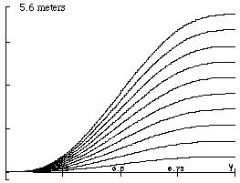 u
u
Figure A.3-1. Ten Maneuvering Curves.
Curvature at u=0 is two, curvature at u=1 is zero.
Figure A.3-1 shows ten curves (y(u) vs. u) for maneuvering through a parking space assuming y0 = 0, dy0 = 0, k0 = 2, dy1 = 0, k1 = 0 and y1 = {1,2...10}. Figure 3.3-2 shows ten curvature curves for the corresponding to the curves of Figure 3.3-1. The end-point curvatures conform to the prescribed k0 = 2 and k1 = 0 constraints.
k(u)
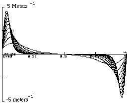
Figure A.3-2. Ten Curvature Curves (k(u) vs. u).
Curvature at u = 0 is two and at u = 1 is zero.

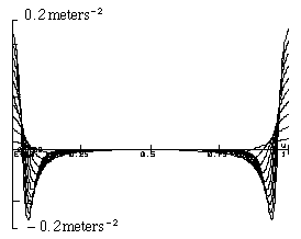
Figure A.3-3. Derivative of the Curvature Function.
These curves give the rate of change curvature with respect to u.
Figure A.3-3 shows the rate of change curvature with respect to u. This gives a notion steering wheel's angular velocity as a function of the path. The steering wheel's angular velocity is limited by factors which have been addressed in Chapter 5.
y
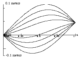
Figure A.3-4. Family of Fifth-order Polynomials.

Figure A.3-4 shows a family of fifth-order polynomials with symmetric end-point slopes. This shows some curve possibilities available for different maneuvering situations. The only constraints used to generate the figure are on the position and slope of the maneuver end-points: the maximum curvature varies from curve to curve.
A system is holonomic when the equations of constraint involve time derivatives of the coordinates that can be integrated to lead to equations involving coordinates only. A system is nonholonomic when the equations of constraint cannot be integrated. A characteristic of a nonholonomic system is that the number of parameters exceeds the number of degrees of freedom. The excess is equal to the number of non-integrable equations of constraint [Korenev 1967] [Fox 1987].
A car is an autonomous mobile robot with nonholonomic constraints because the tires of the car roll so that the point of contact with the road is at rest with respect to the road. The conditions for this to be the case must necessarily involve velocity terms.
For example, if a wheel rolls in a horizontal plane so that it cannot slip sideways, we must have the constraint:
 .
.
The tuple (x,y,[[theta]]) defines the position and orientation of the wheel as shown in Figure B-1.

Figure B-1. A Wheel Perpendicular to a Plane.
Since the wheel does not slip, the rate of change of orientation with respect to time is related to the velocity.
The equation is not integrable and a system constrained by this equation is nonholonomic. While the system has two degrees of freedom, the dynamic specification requires x, y and [[theta]].
Since the wheel does not slip, the rate of change of orientation with respect to time is related to the velocity. The no-slip condition requires that the velocity of the wheel be along the main axis of the wheel. Let s denote the magnitude of this velocity. Then the x component of the velocity is
(a)

and the y component of the velocity is
(b)

Combining (a) and (b) results in the nonholonomic constraint
(c)

Nonholonomic-dynamical systems arise whenever there are non-integrable relations between coordinates and their time derivatives.
 (C.1)
(C.1)
where
FDba5()Sdo5(d) is the force of drag,
FDba5()Sdo5(g) is the force due to gravity,
R is the tire radius and
C is the coefficient of rolling resistance.
For pneumatic tires on a smooth road C = 0.635 mm [Shames 1980]. For the field test vehicle R = 300 mm and mass is 1800 kg so that
FDba5()Sdo5(g) = 1800 kg * 9.8 m/s2 = 17640 kg m/s2
and
FDba5()Sdo5(d) = 17640 kg m/s2 * 0.635 mm/300 mm = 37 kg m/s2.
Engine torque in the Blazer simulation during acceleration[11] is
2829 kg m/s2. Thus the force
due to drag is about 1% of the engine torque during acceleration and is
therefore negligible.
Using four graphic primitives which represent specific formulae, complex models may be represented. The underlying formulae consists of time-varying, non-linear systems of difference equations. The four basic primitives are shown in Figure D-1.
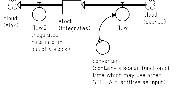
Figure D-1. The Four Basic Modeling Primitives.
Shown are the stock, two flows (with clouds at each end), a converter and an arc connecting a converter with a flow. The arc is used to connect the modeling primitives.
The stock represents a discrete-time integrator and corresponds to a system state variable. The flow regulates the rate into and out of a stock or, in Figure D-1, a cloud. The clouds are infinite sources or sinks and replace the stocks when in-flow or out-flow is not important to the process. The converter provides a place holder for a formula whose inputs and outputs are real numbers of finite precision that may be causally related to other STELLA quantities. An arc between a converter and the flow shows a causal relation.
STELLA is a discrete-time simulator which models continuous-time and discrete-time systems. Continuous-time systems are often modeled with differential equations and STELLA must approximate differential equations with difference equations.
When performing a STELLA simulation there is a starting time and an ending time. Suppose the starting time is zero and the ending time is T. Divide the time interval, 0 <= t <= T into N equal increments, [[Delta]]t. Then

where
 .
.
Assume that [[Delta]]t is small enough so that the simulation signals can be approximated by a piecewise-constant function that changes only at the instants t = 0,[[Delta]]t,...,(N-1)[[Delta]]t; thus, for t = i[[Delta]]t

x(i[[Delta]]t) is referred to as the ith value of x and is denoted by x(i). Rewriting we obtain
 .
.
Stock(i+1) = Stock(i) + [[Delta]]t* Flow(i).
Solving for the flow results in
Flow(i) = (Stock(i+1)-Stock(i))/[[Delta]]t.
In the limit, as [[Delta]]t goes to zero, the difference equation becomes the differential equation:
f(d(Stock(t)),dt) = Flow(t).
For example, if xs = displacement, ks = Hooke's spring constant and ms = mass, then the 2nd-order harmonic oscillator (for a spring-mass system) results:

or

with
 .
.
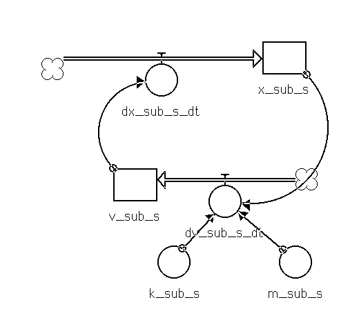
Figure D.1-1. Second Order Harmonic Oscillator.
The two coupled stocks represent two coupled first-order differential equations.
Figure D.1-1 shows the four types of symbols mentioned in the previous section, stocks, converters, flows and clouds.
A run of the model produces Figure D.1-2.
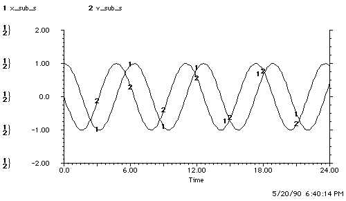
Figure D.1-2. A Second Order Harmonic Oscillator.
The time and date in the lower right corner of the illustration is retained in STELLA graphs.
Figure D.1-2 shows artifacts of the digital approximation to the curves manifested by jaggies. In this simulation, [[Delta]]t = 0.125.

is asymptotically stable [Boyce et al. 1977]. What happens if the system starts at (2,-2) and is constantly perturbed by zero-mean uniform noise? Figure D.2-1 shows the model implemented in STELLA. Random is a STELLA function which generates a series of non-replicable random numbers uniformly distributed between zero and one. To obtain a zero-mean uniform noise source we bias the random function by -0.5.
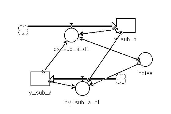
Figure D.2-1. A Model of a Non-Linear 2nd-Order Differential Equation.
The two STELLA stocks represent the two coupled differential equations with noise.
The state equations given to STELLA follow:
x_sub_a = x_sub_a + dt * ( dx_sub_a_dt )
INIT(x_sub_a) = 2
y_sub_a = y_sub_a + dt * ( dy_sub_a_dt )
INIT(y_sub_a) = -2
dx_sub_a_dt = noise-x_sub_a-x_sub_a*y_sub_a^2
dy_sub_a_dt = -noise-y_sub_a-y_sub_a*x_sub_a^2
noise = RANDOM-.5
Figure D.2-2 shows the simulation results.
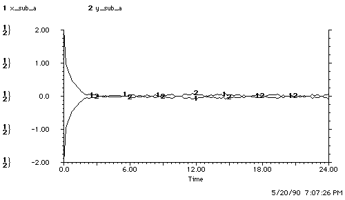
Figure D.2-2. Graph of Stochastic Non-linear, Coupled-Differential Equations.
Analytic results for such systems are elusive.
STELLA can solve initial-value problems in non-linear stochastic systems of differential equations. It is also a simulator that allows the design of controllers through experiment.
ASubSMax [[equivalence]] maximum linear acceleration used by the plant model (asmax)
ASubSMin [[equivalence]] minimum linear acceleration used by the plant model (asmin)
AdjPhi20 [[equivalence]] plant model steering-wheel angle adjusted by the internal sensor at 20 hz with 10% error
Alpha [[equivalence]] proportional to derivative mix ratio for control ([[alpha]])
AlphaSubPhi [[equivalence]] mix ratio for orientation vs. steering-wheel angle ([[alpha]][[phi]])
ApproxDsDtP5 [[equivalence]] linear approximation of the speed of the car based on the 5 hz external sensor sampling of the X and Y coordinates of the plant
ApproxDxDtP5 [[equivalence]] derivative of the externally sampled plant X-coordinate
ApproxDyDtP5 [[equivalence]] derivative of the externally sampled plant Y-coordinate
ASubPhi [[equivalence]] applied plant model steering acceleration in rad/s2
BackupLightsBin [[equivalence]] 1 if backing up, 0 otherwise
Clk5 [[equivalence]] 5 hz clock
Clk5_2dt [[equivalence]] 5 hz clock delayed by two simulator time intervals
Clk5Dt [[equivalence]] 5 hz clock delayed by one simulator time interval
Clk20 [[equivalence]] 20 hz clock
Clk20_2dt [[equivalence]] 20 hz clock delayed by two simulator time intervals
Clk20Dt [[equivalence]] 20 hz clock delayed by one simulator time interval
ControlError [[equivalence]] amount the plant model acceleration parameters are off, expressed as a real which varies from 0 to 1 where 0 is no error and .25 is -25% error. A 1 will eliminate all control and the car will go nowhere. For example, in the steering system: ASubPhiSubP = ASubPhi * (1 - ControlError) * Steering Mode.
DSubBHat [[equivalence]] estimated distance needed to stop the plant as computed by the controller (db)
DdphiDdt [[equivalence]] ASubPhi plant model steering acceleration
Dphi5Dt [[equivalence]] numerically approximated derivative of the reference path steering-wheel angle
DphiDt [[equivalence]] rate of change of the steering-wheel angle of the plant model relative to its longitudinal centerline (f(d[[phi]],dt))
DsDt_1dt [[equivalence]] speed of the front of the plant model delayed by one simulator time interval
DsDtHat [[equivalence]] observer's reconstruction of the velocity of the front
of the plant which may use feedback (Sdo6(
 ))
))
Dtheta5Dt [[equivalence]] derivative with respect to time of the orientation prescribed by the fifth-order polynomial taking the nonholonomic orientation constraint into account (f(d[[theta]]5,dt))
DthetaDt [[equivalence]] rate of change of the plant model orientation
(Sdo10(
 ))
))
DthetaDtHat [[equivalence]] observer's estimate of the rate of change of the
plant's orientation with respect to time (Sdo6(
 ))
))
DthetaDtSubP [[equivalence]] rate of change of the plant orientation with respect to time
DxDtSubP [[equivalence]] X-component of the front of the plant velocity
DyDtSubP [[equivalence]] Y-component of the front of the plant velocity
[[Epsilon]] [[equivalence]] error signal used to steer the plant (e)
ESubDthetaDt [[equivalence]] difference between the observer estimate of the
derivative with respect to time of the plant's steering-wheel angle and the
reference path generator's (sdo10(
 ))
))
ESubTheta [[equivalence]] error contribution of the car orientation to the
steering control error (sdo6(
 ))
))
FeedbackMode [[equivalence]] controls the mode of observer estimation.
Closed loop sensor fusion [[equivalence]] 0,
open-loop plant model based
estimation[[equivalence]]1,
error-free sensing of the
plant[[equivalence]]2,
dead reckoning based estimation[[equivalence]]3,
external sensor based estimation[[equivalence]]4.
In feedback mode 5
the phi5 of the fifth-order polynomial is fed directly into the plant and the
plant is sensed directly by the observer. Invalid feedback modes will yield
wrong results.
Feedback mode is used in phi_hat, s_hat, theta_hat,
ds_dt_hat and phi sub p2
five [[equivalence]] rate, in hz, at which the external sensors sample
FWAError [[equivalence]] internal sensor error of 10%
K5SubB [[equivalence]] curvature of the fifth-order polynomial for moving backward (kb)
K5SubF [[equivalence]] curvature of the fifth-order polynomial for moving forward. The curvature for moving forward is a mirror image about the X-axis of the curvature for moving backward (kf)
L [[equivalence]] length of the car in meters
LinearAccFactor [[equivalence]] a dimensionless number used to vary the maximum 1-D acceleration. 1-D acceleration is linearly proportional to the LinearAccFactor and this factor must vary from [0..1]
OdSubP20 [[equivalence]] 20 hz internal sensor sampling of the odometer
OdSubP20Dt [[equivalence]] one simulator time interval delay of the odometer
OdometerError [[equivalence]] erroneous sensor reading of -10%
Phi [[equivalence]] front wheel angle relative to the longitudinal centerline of the plant model ([[phi]])
Phi5 [[equivalence]] reference path steering-wheel angle, in radians ([[phi]]5)
PhiDt [[equivalence]] plant-model steering-wheel angle delayed by one simulator time interval
PhiSubP20 [[equivalence]] 20 hz internal sensor sampling of the plant's steering-wheel angle, in radians, measured with respect to the main axis of the car
PhiSubP20Dt [[equivalence]] one simulator time interval delay on the 20 hz steering-wheel angle
PhiHat [[equivalence]] a feedback mode sensitive estimation of plant
steering-wheel angle (
 )
)
PhiSubP [[equivalence]] steering-wheel angle of the plant relative to its longitudinal centerline ([[phi]]p )
PSLMinusL [[equivalence]] parking space length minus the car length. Also called the maneuver room (PSL-L)
S [[equivalence]] length of the path traveled by the plant-model (s)
SDt [[equivalence]] path-length of the front wheel of the plant model delayed by one simulator time interval
SteeringMode [[equivalence]] if 0 the steering is on, if 1 the steering is off
SHat [[equivalence]] feedbackmode sensitive reconstruction of the length of the
path traced by the front wheel of the car (
 )
)
SSub_5f [[equivalence]] function which linearly interpolates the length of the path traced by the front of the plant given PSL-L.
SSubP [[equivalence]] an internal sensor (odometer) output which measures the length of the path traveled by the plant front-wheel (sp)
SteeringAccFactor [[equivalence]] dimensionless number used to vary the maximum steering acceleration. Steering acceleration is linearly proportional to the steering acceleration factor and this factor must vary from [0..1]
Theta [[equivalence]] plant model orientation, angle formed by the main axis of the plant with the X-axis of a Cartesian coordinate frame aligned with the curb ([[theta]])
Theta5 [[equivalence]] orientation of the car as given by the fifth-order polynomial ([[theta]]5)
ThetaDt [[equivalence]] plant-model orientation delayed by one simulator time interval
ThetaSubP5 [[equivalence]] 5 hz sample-and-hold on the plant orientation
ThetaHat [[equivalence]] mode sensitive observer reconstruction of the plant
orientation (
 )
)
ThetaSubP [[equivalence]] plant orientation
XP5Dt [[equivalence]] 5 hz sample-and-hold on the plant X-coordinate delayed by one simulator time interval
XSubP5 [[equivalence]] 5 hz sample-and-hold on the plant X-coordinate (xp)
xSubP [[equivalence]] X-position of the front of the plant
YSubP5 [[equivalence]] 5 hz sample-and-hold on the plant Y-coordinate (yp)
ye [[equivalence]] function which linearly interpolates the deflection of the fifth-order polynomial given PSL-L
yrSubP [[equivalence]] Y-position of the rear of the plant
ySubP [[equivalence]] Y-position of the front of the plant

Figure D.5-1. 1-D Plant Model with Longitudinal Controller.
The 1-D observer estimates the distance needed to brake the car.

Figure D.5-2. The STELLA Diagram of the Plant.
The 2-D Front and rear computations for the plant include the nonholonomic constraints. This enables the computation of the plant orientation (ThetaSubP) which supplies the key information for computing the location of the rear of the plant (xrSubP, yrSubP).

Figure D.5-3. The Reference Path Generator, Steering Controller and Plant Model.
The plant model steering system consists of two integrators which accumulate the steering bangs applied by the steering controller (ASubPhi). The steering controller uses the reference steering wheel angle (phi5) and the reference orientation (theta5) to compute the steering control law.

Figure D.5-4. Sensors, Clocks and Fusion.
The internal sensors sample at 20 hertz, the external sensors sample at 5 hertz. The two system clocks run at 5 and 20 hertz. The sensor fusion is between the two external sensors on position and the odometer.

Figure D.5-5. Feedback Mode Logic, the Control Panel and Fusion.
The feedback mode logic is used to control how the observer performs sensor fusion. The control panel organizes key converters for the STELLA operator.

Figure D.5-6. 1 and 2-D Sensor Fusion in the Observer.
The plant model and sensor data are fused using both the internal and external sensors.
The STELLA converters, flows and stocks each contain STELLA formulae. The STELLA formulae for Figure D.5-1 through D.5-6 follows:
AdjS5(t) = AdjS5(t - dt) + (AdjDsDt5) * dt
INIT AdjS5 = 0
AdjDsDt5 = DsDt+adj_ds_dt_error_5
adj_ds_dt_error(t) = adj_ds_dt_error(t - dt) + (adj_ds_dt_g) * dt
INIT adj_ds_dt_error = 0
adj_ds_dt_g = Clk5Dt*(ds_dt_error-adj_ds_dt_error)
adj_ds_dt_error_5(t) = adj_ds_dt_error_5(t - dt) + (adj_ds_dt_g_5) * dt
INIT adj_ds_dt_error_5 = 0
adj_ds_dt_g_5 = Clk5Dt*(DsDtError5-adj_ds_dt_error_5)
adj_phi_error(t) = adj_phi_error(t - dt) + (adj_phi_g) * dt
INIT adj_phi_error = 0
adj_phi_g = clk20_dt*(phi_error-adj_phi_error)
adj_s_error(t) = adj_s_error(t - dt) + (adj_s_g) * dt
INIT adj_s_error = 0
adj_s_g = clk20_dt*(s_error-adj_s_error)
adj_theta_error(t) = adj_theta_error(t - dt) + (adj_theta_g) * dt
INIT adj_theta_error = 0
adj_theta_g = Clk5Dt*(theta_error-adj_theta_error)
Alpha(t) = Alpha(t - dt)
INIT Alpha = .05
AlphaSubPhi(t) = AlphaSubPhi(t - dt)
INIT AlphaSubPhi = 2
BackupLightsReal(t) = BackupLightsReal(t - dt) + (dbu_dt) * dt
INIT BackupLightsReal = 0
dbu_dt = if (BackupLightsBin=0) and (SHat>=PSLMinusL) then 1/dt else if (BackupLightsBin=1) and (SHat<=bu_obj_psn) then -BackupLightsReal/dt else 0
ControlError(t) = ControlError(t - dt)
INIT ControlError = .25
DphiDt(t) = DphiDt(t - dt) + (ddphi_ddt) * dt
INIT DphiDt = 0
ddphi_ddt = ASubPhi
DphiDtSubP(t) = DphiDtSubP(t - dt) + (DdphiDdtSubP) * dt
INIT DphiDtSubP = 0
DdphiDdtSubP = ASubPhiSubP
DsDt(t) = DsDt(t - dt) + (DdsDdt) * dt
INIT DsDt = 0
DdsDdt = ASubS
DsDtSubP(t) = DsDtSubP(t - dt) + (DdsDdtSubP) * dt
INIT DsDtSubP = 0
DdsDdtSubP = ASubSSubP
ds_dt_s_error_20(t) = ds_dt_s_error_20(t - dt) + (adj_ds_dt_g_20) * dt
INIT ds_dt_s_error_20 = 0
adj_ds_dt_g_20 = clk20_dt*(ds_dt_error_20-ds_dt_s_error_20)
FeedbackMode(t) = FeedbackMode(t - dt)
INIT FeedbackMode = 0
od_sub_p20(t) = od_sub_p20(t - dt) + (od_sample) * dt
INIT od_sub_p20 = 0
od_sample = clk20*(odometer_error-od_sub_p20)
Phi(t) = Phi(t - dt) + (SteeringSpeed) * dt
INIT Phi = 0
SteeringSpeed = DphiDt
PhiSubP(t) = PhiSubP(t - dt) + (SteeringSpeedSubP) * dt
INIT PhiSubP = 0
SteeringSpeedSubP = DphiDtSubP
phi_sub_p20(t) = phi_sub_p20(t - dt) + (phi_sample) * dt
INIT phi_sub_p20 = 0
phi_sample = clk20*(fwa_error-phi_sub_p20)
s(t) = s(t - dt) + (LinearSpeed) * dt
INIT s = 0
LinearSpeed = DsDt
SingleManeuverMode(t) = SingleManeuverMode(t - dt)
INIT SingleManeuverMode = 1
SSubP(t) = SSubP(t - dt) + (LinearSpeedSubP) * dt
INIT SSubP = 0
LinearSpeedSubP = DsDtSubP
SteeringMode(t) = SteeringMode(t - dt)
INIT SteeringMode = 1
Theta(t) = Theta(t - dt) + (DthetaDt) * dt
INIT Theta = 0
DthetaDt = DsDtHat*sin(PhiHat)/L
theta5(t) = theta5(t - dt) + (Dtheta5Dt) * dt
INIT theta5 = 0
Dtheta5Dt = DsDtHat*sin(phi5)/L
ThetaSubP(t) = ThetaSubP(t - dt) + (DthetaDtSubP) * dt
INIT ThetaSubP = 0
DthetaDtSubP = DsDtSubP*sin(Phi2SubP)/L
theta_sub_p5(t) = theta_sub_p5(t - dt) + (theta_sample) * dt
INIT theta_sub_p5 = 0
theta_sample = clk5*(ThetaSubP-theta_sub_p5)
xSubP(t) = xSubP(t - dt) + (DxDtSubP) * dt
INIT xSubP = 0
DxDtSubP = DsDtSubP*cos(ThetaSubP+Phi2SubP)
x_sub_p5(t) = x_sub_p5(t - dt) + (x_sample) * dt
INIT x_sub_p5 = 0
x_sample = clk5*(xSubP-x_sub_p5)
YSubP(t) = YSubP(t - dt) + (DyDtSubP) * dt
INIT YSubP = 0
DyDtSubP = DsDtSubP*sin(ThetaSubP+Phi2SubP)
y_sub_p5(t) = y_sub_p5(t - dt) + (y_sample_2) * dt
INIT y_sub_p5 = 0
y_sample_2 = clk5*(YSubP-y_sub_p5)
AdjPhi20 = Phi+adj_phi_error
AdjS20 = s+adj_s_error
AdjTheta5 = Theta+adj_theta_error
adj_ds_dt_20 = DsDt+ds_dt_s_error_20
adj_ds_dt_20_1dt = DELAY(adj_ds_dt_20,DT)
approx_ds_dt_p20 = (od_sub_p20-DELAY(od_sub_p20,1/20))/(1/20)
approx_ds_dt_p5 = if adj_ds_dt_20<0 then -sqrt(approx_dx_dt_p5^2+approx_dy_dt_p5^2) else sqrt(approx_dx_dt_p5^2+approx_dy_dt_p5^2)
approx_dx_dt_p5 = (x_sub_p5-DELAY(x_sub_p5,1/5))/(1/5)
approx_dy_dt_p5 = (y_sub_p5-DELAY(y_sub_p5,1/5))/(1/5)
ASubPhi = if e < 0 then ASubPhiMax else -ASubPhiMax
ASubPhiMax = 50*SteeringAccFactor
ASubPhiSubP = ASubPhi*(1-ControlError)*SteeringMode
ASubS = if SingleManeuverMode=1 then
if DsDtHat < 0 then 0
else forward_acc_command
else
if BackupLightsBin=0 then forward_acc_command
else backup_acc_command
ASubSMax = .83*LinearAccFactor
ASubSMin = 1.4*LinearAccFactor
ASubSMinSubP = ASubSMin *(1-ControlError)
ASubSSubP = if SingleManeuverMode=1
then if DsDtSubP < 0
then 0
else if DsDtSubP>0 and FeedbackMode = 1 and PlantBackwardAcceleration=0 then -ASubSMinSubP else PlantForwardAcceleration
else if BackupLightsBin=1
then PlantBackwardAcceleration
else PlantForwardAcceleration
BackupLightsBin = if BackupLightsReal > 0 then 1 else 0
backup_acc_command = if SHat<=bu_obj_psn then 0 else if SHat-DSubBHat<=bu_obj_psn then ASubSMin else -ASubSMax
bu_obj_psn = 0
clk20 = pulse(1, 0, 1/twenty)
clk20_2dt = DELAY(clk20,2*dt)
clk20_dt = DELAY(clk20,dt)
clk5 = pulse(1, 0, 1/five)
Clk5Dt = DELAY(clk5,DT)
clk5_2dt = DELAY(clk5,2*dt)
dphi5_dt = (phi5-DELAY(phi5,DT))/DT
DsDtDt = DELAY(DsDt,DT)
DsDtError5 = approx_ds_dt_p5-DsDtDt
DsDtHat = if FeedbackMode = 0 then FusedDsDt else if FeedbackMode = 1 then DsDt else if FeedbackMode=2 then DsDtSubP else if FeedbackMode=3 then adj_ds_dt_20 else if FeedbackMode=4 then AdjDsDt5 else if FeedbackMode=5 then DsDtSubP else 0
DSubBHat = (DsDtHat^2)/(2* ASubSMin)
ds_dt_1dt = DELAY(DsDt,DT)
ds_dt_error = approx_ds_dt_p5-adj_ds_dt_20_1dt
ds_dt_error_20 = approx_ds_dt_p20-ds_dt_1dt
DthetaDtHat = DsDtHat*sin(PhiHat)/L
e = eSubPhi+AlphaSubPhi*e_sub_theta
eSubPhi = PhiHat-phi5 +Alpha*(DphiDt-dphi5_dt)
e_sub_dtheta_dt = DthetaDtHat-Dtheta5Dt
e_sub_theta = if BackupLightsBin=1 then -(ThetaHat-theta5+Alpha*e_sub_dtheta_dt) else ThetaHat-theta5+Alpha*e_sub_dtheta_dt
five = 5
forward_acc_command = if SHat+DSubBHat >= PSLMinusL then -ASubSMin else ASubSMax
FusedDsDt = adj_ds_dt_20+adj_ds_dt_error
fwa_error = PhiSubP*.9
k5SubB = (120*ye*(PSLMinusL-SLim)^3/PSLMinusL^5-180*ye*(PSLMinusL-SLim)^2/PSLMinusL^4+60*e*(
PSLMinusL-SLim)/PSLMinusL^3)/((30*ye*(PSLMinusL-SLim)^4/PSLMinusL^5-60*ye*(PLMinusL-SLim)^3
/PSLMinusL^4+30*ye*(PSLMinusL-SLim)^2/PSLMinusL^3)^2+1)^(3/2)
k5SubF = (120*ye*SLim^3/PSLMinusL^5-180*ye*SLim^2/PSLMinusL^4+60*ye*SLim/PSLMinusL^3)/((3
*ye*SLim^4/PSLMinusL^5-60*ye*SLim^3/PSLMinusL^4+30*ye*SLim^2/PSLMinusL^3)^2+)^(
3/2)
L = 2.6
LinearAccFactor = 1
odometer_error = SSubP*.9
od_sub_p20_dt = DELAY(od_sub_p20,DT)
Phi2SubP = if FeedbackMode=5 then phi5 else PhiSubP
phi5 = if BackupLightsBin=1 then ARCTAN(k5SubB*L) else ARCTAN(k5SubF*L)
PhiHat = if FeedbackMode = 0 then AdjPhi20 else if FeedbackMode = 1 then Phi else if FeedbackMode=2 then PhiSubP else if FeedbackMode=3 then AdjPhi20 else if FeedbackMode=4 then Phi else if FeedbackMode=5 then PhiSubP else 0
phi_dt = DELAY(Phi,DT)
phi_error = phi_sub_p20-phi_dt
phi_sub_p20_dt = DELAY(phi_sub_p20,DT)
PlantBackwardAcceleration = if ASubS<0 then ASubS*(1+ControlError) else ASubS*(1-ControlError)
PlantForwardAcceleration = if ASubS>0 then
ASubS*(1+ControlError) else
ASubS *(1-ControlError)
PSLMinusL = 2.4
SHat = if FeedbackMode = 0 then AdjS20 else if FeedbackMode = 1 then s else if FeedbackMode=2 then SSubP else if FeedbackMode=3 then AdjS20 else if FeedbackMode=4 then AdjS5 else if FeedbackMode=5 then SSubP else 0
SLim = if SHat < 0 then 0 else if SHat > PSLMinusL then PSLMinusL else SHat
SteeringAccFactor = 1
s_dt = DELAY(s,dt)
s_error = od_sub_p20-s_dt
ThetaHat = if FeedbackMode = 0 then AdjTheta5 else if FeedbackMode = 1 then Theta else if FeedbackMode=2 then ThetaSubP else if FeedbackMode=3 then Theta else if FeedbackMode=4 then AdjTheta5 else if FeedbackMode=5 then ThetaSubP else 0
theta_dt = DELAY(Theta,DT)
theta_error = theta_sub_p5-theta_dt
twenty = 20
xrSubP = xSubP-L*cos(ThetaSubP)
x_p5_dt = DELAY(x_sub_p5,dt)
YrSubP = YSubP-L*sin(ThetaSubP)
s_sub_5f = GRAPH(PSLMinusL)
(0.00, 0.00), (1.00, 1.11), (2.00, 2.23), (3.00, 3.37), (4.00, 4.54), (5.00, 5.74), (6.00, 6.98), (7.00, 8.28), (8.00, 9.65), (9.00, 11.1), (10.0, 12.6)
ye = GRAPH(PSLMinusL)
(0.00, 0.00), (1.00, 0.0392), (2.00, 0.158), (3.00, 0.357), (4.00, 0.642), (5.00, 1.02), (6.00, 1.49), (7.00, 2.06), (8.00, 2.75), (9.00, 3.55), (10.0, 4.49)
The this code is sufficient to reproduce the STELLA simulation using STELLA or some other computer language or simulator (after some translation).
 (4.16)
where
 (4.17),
 (4.18),
and
 (4.19).
With the variable, backup_lights, is set equal to one when the car is backing up. The values
 (4.20)
were said to give good results.
Since the values in (4.20) are central to the control of the car, we spend the remaining portion of this appendix summarizing the experiments which led to their choice. The closed-loop simulation of Chapter 5 is used to establish the best choice for the values in (4.20). The L1 error [Matthews 1987] is used to establish a figure of tracking merit The L1 error is given by:
 (E.1).
For a single maneuver, N=400 time intervals of 0.01 seconds (four seconds of real-time). If the L1 error is divided by N the result is the average error.
There are three plant states of concern, the orientation, the steering wheel angle and the overshoot. The range of (4.20) used is given by:
 (E.2).
Over the range in (E.2) the overshoot varied by less than 0.01 meters and so was not a factor in selecting (4.20). Figure E-1. summarizes the experimental results.


 0.05 0 0.136 0.146
0.05 2 0.046 0.154
0.05 4 0.050 0.214
0 2 0.041 0.263
0.03 2 0.047 0.138
0.05 2 0.046 0.154
0.07 2 0.053 0.177
0.10 2 0.056 0.199
Figure
E-1. Summary of the L1 Errors for Various Mix RatiosDividing the L1 error by N=400 results in the average error. The maximum average error over the range in (E.2) is in the steering-wheel tracking and is 0.0006575 radians.
There are no known analytic arguments for a specific mix ratio for such a non-linear system. The only justification for the choices of the mix ratio must therefore be made via experiment. The average error is so small in the range selected (E.2) that it hardly matters if (4.20) is off a little. The reader should note, however, that range was arrived at after many more experiments than reported in Figure E-1.
Assume that the car is subject to the closed-loop sensor fusion, sensor error and modeling error described in Chapter 5. Using a modeling error of 25% several experiments are run using various PSL-L's. The result is shown in Figure F-1.
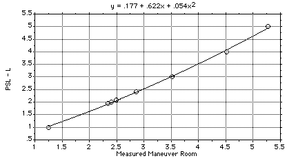
Figure F-1. PSL-L vs. Measured Maneuver Room.
A quadratic best-fit polynomial approximation to the data gives a handy means of computing the PSL-L given the maneuver room measurement. All measurements are in meters.
The overshoot varies from 20% to 4% (as measured maneuver room varies from 1.25 to 5.25 meters). The reason is that braking distance (4.5) has a constant acceleration modeling error and a quadratic velocity error. For small maneuvers the velocity is low and the constant error dominates. For large maneuvers the velocity is high and the velocity error dominates.
If the modeling error exceeds 25% overshoot will increase and Figure F-1 must be recomputed or a collision will occur. If the modeling error is less than 25% we will not be taking full advantage of the available maneuver room.
 (= linear acceleration of Chapter 4) is multiplied by the acceleration
factor.
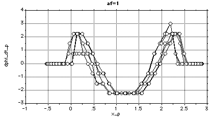
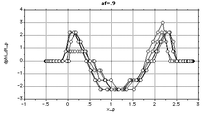
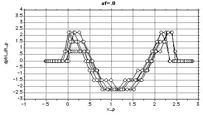
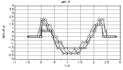
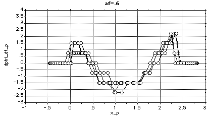
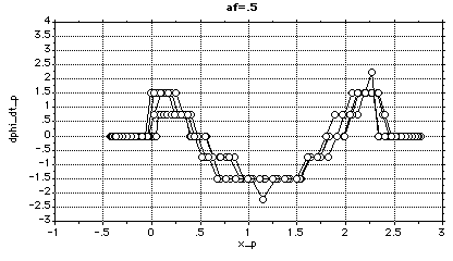
Figure G-1. Linear Acceleration vs. Steering Speed.
Dphi_dt_p is the steering speed of the plant in radians per second. X_p is the x-position of the plant in meters. Af is the acceleration factor which is used to reduce the linear acceleration of the plant.
Figure G-1 shows that the steering velocity takes on discrete values, due to the bang-bang control used on the steering, and that the maximum steering velocity varies from 3 radians per second to 2.25 radians per second. Figure G-1 also shows that the effect of changing the linear acceleration of the plant on the steering speed is small.
Modeling ErrorFigure H-1. Modeling Error vs. Plant Performance.Radians
Radians X-Deflection when speed is zero 0% .043 .136 2.41 m 5% .045 .131 2.48 m 10% .045 .132 2.55 m 15% .045 .135 2.62 m 20% .044 .136 2.75 m 25% .046 .154 2.86 m
Dividing the L1 error by N=400 results in the average error. The maximum average error over the range in (H-1) is in the steering-wheel tracking and is 0.000385 radians.
It is evident from Figure H-1 that orientation and steering-wheel tracking have small change in L1 error as modeling error is varied. The overshoot has a much larger change, however.
controller [[equivalence]] software which receives plant-state estimates formulated by the observer and which issues commands to the plant model and the plant.
converter [[equivalence]] a STELLA construct that transforms its input according to a given formula. It is represented by a circle.
dead reckoning [[equivalence]] position estimation by the observer using only internal sensors and the plant model.
external sensor [[equivalence]] a device which measures plant states relative to the environment. In this thesis, the external sensor references are to software which models an external sensor.
flow [[equivalence]] a STELLA pipe that represents a differential quantity directed into or out of a stock.
front-wheel [[equivalence]] a part of the car which both steers and propels the car. When referring to front-wheel's steering parameters it is called the steering-wheel and is given in radians and seconds (i.e., steering-wheel angle, steering-wheel angular velocity and steering-wheel angular acceleration). When referring to the front-wheel's propelling parameters it is called the front-wheel and is given in meters and seconds (i.e., front-wheel path length, front-wheel velocity and front-wheel acceleration).
internal sensor [[equivalence]] a device which measures plant states relative to the plant. In this thesis, the internal sensor references are to software which models an internal sensor.
observer [[equivalence]] software which receives plant-model states and (if closed-loop) sensor feedback. Its output is a plant-state estimate.
plant [[equivalence]] software which is assumed to correctly model a car. The plant receives controller commands and its state variables are measured by sensors.
plant model [[equivalence]] software which models (possibly incorrectly) a car. The plant model reacts to controller commands and its state variables are used by the observer.
STELLA [[equivalence]] Structural Thinking Experimental Learning Laboratory with Animation, discrete event simulator.
stock [[equivalence]] a STELLA building block that integrates the output of a flow. A stock is diagrammed as a rectangle.
front path [[equivalence]] the path traced by the front of the car.
rear path [[equivalence]] the path traced by the rear of the car.
 the proportional to derivative mix ratio for control.
sdo7(
 )
the mix ratio for orientation vs steering-wheel angle.
sdo4(
 )
maximum 1-D acceleration for the plant model.
sdo6(
 )minimum 1-D acceleration for the plant model. This is a negative quantity.
[[Delta]]t [[equivalence]] simulator time interval.
kmax [[equivalence]] the magnitude of the minimum turning radius of the rear of the plant.
L [[equivalence]] length of the plant and plant model.
PSL [[equivalence]] Parking Space Length (equal to the distance between the car in front and the car in back).
PSW [[equivalence]] the Parking Space Width (assume that this is large).
xe[[equivalence]] PSL-L [[equivalence]] X-component of the end-point of the fifth-order polynomial.
ye [[equivalence]] Y-component of the end-point of the fifth-order polynomial.
 )
1-D acceleration command for the plant model.
sdo9(
 )
1-D acceleration command for the plant.
sdo6(
 )
estimated distance to brake the plant for both forward and backward motion.
This is computed by the controller using observer plant-state estimates and is
used in both 1-D and 2-D operation.
e [[equivalence]] the difference signal used to steer the plant.
sdo19(
 )the
difference between the observer estimate of the derivative with respect to time
of the plant's steering-wheel angle and the reference path generator's.
sdo16(
 )the difference between the observer estimate of the derivative with respect to
time of the plant orientation and the reference path generator's.
sdo6(
 )
weighted contribution of the estimated steering-wheel angle error and its
derivative with respect to time.
sdo6(
 )weighted contribution of the estimated orientation error and its derivative
with respect to time.
k5 [[equivalence]] curvature of the fifth-order polynomial.
sdo4(
 )curvature
of the fifth-order polynomial for moving backward.
sdo4(
 )curvature
of the fifth-order polynomial for moving forward. The curvature for moving
forward is a mirror image about the X-axis of the curvature for moving
backward.
[[phi]] [[equivalence]] steering-wheel angle relative to the longitudinal centerline of the plant model.
sdo4(
 ) the steering-wheel angle of the car when the rear of the car follows a
fifth-order polynomial, without error.
f(d[[phi]],dt) [[equivalence]] rate of change of the steering-wheel angle of the plant model relative its longitudinal centerline.
[[phi]]p [[equivalence]] steering-wheel angle relative to the longitudinal centerline of the plant.
 .
.
r [[equivalence]] turning radius of the front of the car when the rear of the car follows a fifth-order polynomial, without error.
s [[equivalence]] length of the path traveled by the plant-model.
s5 [[equivalence]] length of the path traveled by the front of the car when the rear of the car follows a fifth-order polynomial, without error.
sdo13(
 )front-wheel plant-model speed.
sp [[equivalence]] an internal sensor output which measures the length of the path traveled by the plant front-wheel.
[[theta]] [[equivalence]] plant model orientation, angle formed by the main axis of the plant with the X-axis of a Cartesian coordinate frame aligned with the curb.
[[theta]]5 [[equivalence]] car orientation.when the rear of the car follows a fifth-order polynomial, without error.
f(d[[theta]],dt) [[equivalence]] rate of change of the plant-model orientation.
[[theta]]p [[equivalence]] an external sensor output which measures the plant orientation.
X,Y [[equivalence]] 2-D Cartesian coordinate axis embedded in the plant and aligned with respect to the parking space.
x [[equivalence]] X-component of the front of the plant model.
y [[equivalence]] Y-component of the front of the plant model.
xp [[equivalence]] external sensor output which measures the deflection of the X-component of the front of the plant.
yp [[equivalence]] external sensor output which measures the Y-component of the front of the plant.
xf [[equivalence]] the deflection of the X-component of the front of the car when the rear of the car follows a fifth-order polynomial, without error.
yf [[equivalence]] the Y-component of the front of the car when the rear of the car follows a fifth-order polynomial, without error.
xr [[equivalence]] X-component of the rear of the plant (xr [[epsilon]] [0,PSL-L]).
yr [[equivalence]] Y-component of the rear of the plant.
f(dx,dt) [[equivalence]] rate of change of the X-component of the front of the plant model.
f(dy,dt) [[equivalence]] rate of change of the Y-component of the front of the plant model.
f(dy,dx) [[equivalence]] rate of change of the Y-component of the front of the plant model with respect to its X-component.
sdo12(
 )
rate of change of the Y-component of the rear of the plant model with respect
to X-component of the rear of the plant model.
sdo12(
 )
acceleration of the Y-component of the rear of the plant model with respect to
X-component of the rear of the plant model.
sdo4(
 )estimates made by the observer. For example:
 [[equivalence]] X-component of the front of the plant as estimated by the
observer;
 Y-component
of the plant as estimated by the observer.
ASubSSubP [[equivalence]] sdo9(
 )
1-D acceleration command for the plant.
dds_ddt [[equivalence]] the error-free plant and observer's plant model front-wheel acceleration.
dds_dt_p [[equivalence]] the plant's front-wheel acceleration from open-loop control.
dphi5_ddt [[equivalence]] the steering-wheel angular acceleration when the rear of the car follows a fifth-order polynomial, without error.
dphi_dt [[equivalence]] f(d[[phi]],dt) [[equivalence]] rate of change of the steering-wheel angle of the plant model relative its longitudinal centerline.
ds_dt [[equivalence]] the error-free plant and observer's plant model front-wheel speed.
ds_dt_p [[equivalence]] the front-wheel plant speed from open-loop control.
DsDtSubP [[equivalence]] the front-wheel plant speed from closed-loop control.
OdSubP20 [[equivalence]] 20 hz internal sensor sampling of the odometer.
SHat [[equivalence]] feedbackmode sensitive reconstruction of the length of the
path traced by the front wheel of the car (
 ).
).
SSubP [[equivalence]] sp [[equivalence]] the length of the path traveled by the plant front-wheel.
ThetaHat [[equivalence]] mode sensitive observer reconstruction of the plant
orientation (
 ).
).
ThetaSubP [[equivalence]] plant orientation.
ThetaSubP5 [[equivalence]] 5 hertz sample-and-hold on the plant orientation.
x_p [[equivalence]] X-position of the front of the plant.
xr_p [[equivalence]] X-position of the rear of the plant.
y_p [[equivalence]] Y-position of the front of the plant.
yr_p [[equivalence]] Y-position of the rear of the plant.
dy0 [[equivalence]] initial slope of the fifth-order polynomial.
dy1 [[equivalence]] final slope of the fifth-order polynomial.
k0 [[equivalence]] initial curvature of the fifth-order polynomial.
k1 [[equivalence]] final curvature of the fifth-order polynomial.
t1,t2...t77 [[equivalence]] auxiliary variables introduced by Maple.
u [[equivalence]] auxiliary variable which, when varied from zero to one, inclusive, generates a path.
x0 [[equivalence]] X-component of the start point of the fifth-order polynomial.
y0 [[equivalence]] Y-component of the start point of the fifth-order polynomial.
x1 [[equivalence]] X-component of the end point of the fifth-order polynomial.
y1 [[equivalence]] Y-component of the end point of the fifth-order polynomial.
 .
.
 .
.
FDba5()Sdo5(d) [[equivalence]] force due to rolling resistance.
FDba5()Sdo5(g) [[equivalence]] force due to gravity.
R [[equivalence]] tire radius.
ms [[equivalence]] mass of a spring.
random [[equivalence]] a function used by STELLA to generate a series of values with uniform distribution.
vs [[equivalence]] speed of the spring-mass system.
xa [[equivalence]] X-deflection.
xs [[equivalence]] deflection of the spring-mass system.
ya [[equivalence]] Y-deflection.
L1 Error [[equivalence]] A scalar figure of tracking merit where:
 .
.
N [[equivalence]] number of intervals.
Pk [[equivalence]] plant state at interval k.
Rk [[equivalence]] reference state at interval k.