Performance of Real-time Nth Order Stochastic Compositions[1]
by
Douglas Lyon
E-mail: Lyon@cse.bridgeport.edu
Phone: (203)576-4760
Computer Science and Engineering Department, Dana Building
University of Bridgeport
Bridgeport CT 06601
Abstract
This article presents a technique for the use of stochastic Petri-nets for real-time realization of Nth order stochastic compositions (a Markov process). The algorithm makes use of a data structure known as a stochastic Petri table. This table is compact and suitable for interactive performance on lap-top type computers. We also show how the inherently concurrent nature of Petri nets can be used to implement real-time MIDI processing. Since some readers are unfamiliar with Petri nets, we present a brief and incomplete introduction to the basic ideas behind the Petri net and compare it with the finite state machine.
The use of Markov chains for computer assisted composition is not new, Schwanauer and Levitt's book, Machine Models of Music, describe an experiment performed in 1955 called Illiac Suite. This experiment was performed by Lejaren Hiller and Leonard Isaacson (Schwanauer and Levitt).
Attempts to realize Markov chain performance in real-time are not new (O'Haver 1978). This was only a first-order processes, however. High-order Markov chain composition has not been published in real-time, as far as we know.
A stochastic Petri-table is a data structure that is shown to enable the computation of high-order real-time Markov processes. We encode a melody using pitch class and ignore tempo and timbre information. Tempo and timbre information are ignored in order to simplify the presentation. The computation of the stochastic Petri-table is an off-line process, however, the table is compact (linear in the number of arcs) and enables real-time Markov chain computation. Our brute-force approach to building the Petri-table, while easy to implement, is slow. A harder to implement, but faster approach, has been suggested but remains untried. After the computation of the stochastic Petri-table, the program writes it to a file to be read during program start-up. Thus, this stochastic Petri-net approach allows us to perform a precomputation phase which permits fast execution.
We are motivated to take the stochastic Petri-net approach because we have found approaches in literature which do not give real-time performance and which use more memory than is practical on portable computers (Moore 1990). A further motivation for the use of Petri-nets is the concurrent nature of interfaces and music performance. It is often the case, for example, that a user will create interrupts during a performance. As shown in the following sections, these interrupts cannot be handled with a finite state machine but can be handled by Petri-nets.
A Turing machine is a computing device which consists of a control unit (which may assume one state at a time), a tape (which can store a symbol) and a read-write head (which moves relative to the tape and can relay information between the control unit and the tape).
A finite state machine is a deterministic device with a fixed number of states. A special case of the Turing machine, the finite state machine is also known as a finite automaton. The finite state machine consists of a Turing machine with a single input tape and a read-only head (Ralston 1983). The output and next-state of a finite state machine are a function of the machine's present state and inputs (Katz 1994).
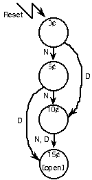
Finite-state machines are often depicted by state diagrams. A state diagram is a directed graph which shows the input and output of the finite state machine. An example of a finite state machine diagram representation of a gum machine is shown in Figure 1.

Figure 1 A Finite State Machine Diagram for a Gum Machine
The price of gum from this machine is 15 cents. The Petri net can represent any finite state machine but the opposite is not true.
The finite state machine model does not handle interrupts well. From a programmer's view, a subroutine is serviced after the state of the machine is pushed onto a stack. The finite state machine does not provide a stack, nor does it describe how an interrupt should be serviced, or to where it should return.
A further limit of the finite state machine model is that it does not handle multiple asynchronous processes. This is really a result of its inability allow for the synchronization of parallel activities. One way to perform this synchronization is through the use of token passing.
Petri nets, which are covered in the following section, are able to model concurrency and interrupts, two features which are notably lacking in the finite state machine.
In the Petri net, places symbolize conditions and transitions symbolize computations. In addition, every transition is connected to input and output places.
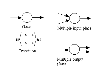
Figure 2 Petri-net Primitives
The Petri-net is a bipartite graph because there are two types of nodes, places and transitions. It is a directed graph because all arcs connect from a place to a transition or from a transition to a place.
The Petri-net may be represented graphically using a Petri-net diagram or it may be represented textually using a Petri-net table. The primitives of the Petri-net diagram are shown in Figure 2. The diagram is better suited for human communication, while the table is better suited for machine communication. Figure 3 shows an example of a Petri net for a gum machine represented by both a Petri-net diagram and a Petri-net table.
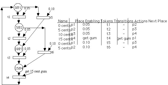
Figure 3 Petri- Diagram and Table for a Gum Machine
The price of gum is 15 cents and no change is given.
The Petri net represented in Figure 3 is modeled with a finite state machine diagram shown in Figure 1. The finite state machine cannot model interrupts, and these are present in the example of a real-time MIDI delay system, shown in Figure 4. The real-time MIDI delay system is designed to act like a 3 second echo box with no decay and a maximum number of echos for every MIDI event. This has several advantages over traditional approaches to achieving a 3 second delay. There is no noise or decay in the repeated event. In addition, the number of echos is a parameter which is settable by the performer.
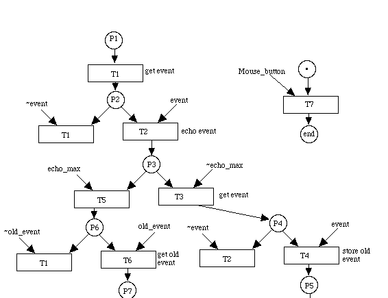
Figure 4 A Petri-Net for a Real-Time 3 Second Midi Delay.
From any place in the Petri net (P1..P7), an interrupt in the main event loop may be generated by the user's input of a mouse click.
The interrupt generated by the user, shown in Figure 4 by the Mouse_button token, is typical of user generated events. User input occurs concurrently with the execution of the main body of the program, and is asynchronous with respect to the execution of the code.
The Petri-net represented in Figure 4 may be represented as a Petri-table and this is shown in Figure 5.
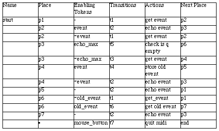
Figure 5 A Petri-Table for a 3 Second Delay
This table represents the same Petri net which is shown by the Petri diagram of Figure 4. The * in the last row, second column of the Petri table indicates that the mouse_button token will cause a jump from any place in the Petri net.
A fragment of Pascal code which implements the Petri-table shown in Figure 5 is given in Figure 6.
begin { of main}
initialize_program;
transition := 1;
repeat
case transition of
1: {scan for an event }
begin
if midi_get(event) then {p1}
transition := 2 {got an event}
else
transition := 1;
end; {case 1}
2: {output note }
begin
echo_event(event);
if event.number_of_times_put < max_echos then
transition := 3
else
transition := 5;
{ok, we echoed enough times, check the queue for old events}
end; {case 2}
3: {update and start again if any new events occur}
begin
if midi_get(event2) then
transition := 4 {a new event occured while we were echoing}
else
transition := 2; {keep echoing, no new inputs}
end; {case 3}
4:
begin
(event); {keep old event for later}
writeln('stashing old event');
copy_event(event2, event);
transition := 2;
end; {case 4}
5:
begin
if q_empty then
transition := 1 {scan for fresh events}
else
transition := 6;
end; {case 5}
6:
begin {queue is not empty so get stashed event and echo it}
remove_q(event);
writeln('removed old event');
transition := 2;
end; {case 6}
end; {case}
until button;
QuitMidi; {discards memory and removes interrupt handlers}
end.
Figure 6. Code For A Three Second Delay
This code was written using Think Pascal(TM) on a Macintosh computer (Symantec 1991). The code was designed to be executed in a sequential fashion and so does not enable the handling of true interrupts. Instead the events are queued by the operating system and de queued by the until button of the main event loop of the program. For the case of parallel Pascal, a more direct translation from the Petri net to the code is possible.
A Markov process (or Markov chain) is a non-deterministic finite state machine. The difference is that there are probabilities assigned to the arcs in the finite state machine diagram. In addition, the sum of all the probabilities leaving any Markov state is equal to one.
A Markov random process is classed as being continuous-valued or discrete-valued. For the purpose of selecting pitches from a scale (finite set), we use the discrete-valued Markov random process (i.e., Markov Chain). A Markov chain is a DVMRP with a countable or finite set of states (Stark and Woods).
The Markov chain satisfies the conditional probability mass function expression
 (1.3-1)

The value of the random variable X at time t will determine the conditional probabilities for the future process values. The process values are called the process state and the conditional probabilities are called the transition probabilities between the states. A Markov process is stationary if the probabilities are static. We assume that the Markov process is stationary because we perform off-line analysis.
The transition table of probabilities uses
 (1.3-2)
The resulting two dimensional table represents the transition probabilities in a first-order Markov chain, as discussed by Dodge and Jerse in their book Computer Music. Dodge and Jerse, like Moore, describe an N+1 dimensioned table to represent an Nth order Markov process (Dodge and Jerse). The brute-force approach to the composition using Markov chains usually centers upon the creation of a transition table.
This table of arc-transition probabilities is usually sparse and so requires a program to perform access and computation with a large high-dimensioned matrix containing many zero elements. The probabilities assigned to the arcs may be arrived at by one of several methods. We use a technique of statistical analysis of an existing piece of music and have found this method described in the literature (Moore 1990).
The order of a Markov process indicates the amount of event memory that the process has. For example, a 0th order Markov process has no event memory. A 1st order Markov process takes into account a single event and an Nth order Markov process takes into account the last N events.
In order to perform the analysis of a melody, we convert the notes of a melody into their corresponding pitch class. For example, in Louis Bonfi's Black Orpheus, the notes are:
E, C, B, A, A, G#, B, E, E, C, B, A, A, G, B, E, E, F, G, A, D, D, D, E, F, G, C, C, C, D, E, F, B, B, C, D, E, E, C, B, A, A, G#, B, E, E, A#, A, G, G, F, E, A, D, D, E, F, G, C, C, D, E, A, G#, E, E, G#, B, A, E, A, A, B, C, D, C, B, A, B, C, D, C, B, A, B, C, D, C, B, A, G.
Converting into a pitch class requires that each note be assigned a number, for example:
[A A# B C C# D D# E F F# G G#] = [1 2 3 4 5 6 7 8 9 10 11 12]
Black Orpheus then becomes:
8, 4, 3, 1, 1, 12, 3, 8, 8, 4, 3, 1, 1, 11, 3, 8, 8, 9, 11, 1, 6, 6, 6, 8, 9, 11, 4, 4, 4, 6, 8, 9, 3, 3, 4, 6, 8, 8, 4, 3, 1, 1, 12, 3, 8, 8, 2, 1, 11, 11, 9, 8, 1, 6, 6, 8, 9, 11, 4, 4, 6, 8, 1, 12, 8, 8, 12, 3, 1, 8, 1, 1, 3, 4, 6, 4, 3, 1, 3, 4, 6, 4, 3, 1, 3, 4, 6, 4, 3, 1, 11.
The technique of converting a melody into its corresponding pitch class is not new (Winsor 1987). These notes are placed into a file, called notes and read into an array of integers called note_array[i].
 (1.3-3)
Assume that the occurrence of a note is an independent random event. We have written a procedure which compiles a table that records the frequency of occurrence into an array called the pmf_array[i]. Here, PMF is an abbreviation for the probability mass function. This is a statistical record of the frequency of occurrence of each note in the melody. It is treated as a discrete probability distribution function so that
 (1.3-4)
must be true.
We use the probability mass function array to bias our choice of a note by picking a random number, random_pick such that
 .
(1.3-5)
We then compute the cumulative mass function by summing the elements of the probability mass function array until they exceed random_pick. This is shown in the following pseudo code.
Compute the probability mass function array, pmf_array
random_pick = random(0,1)
sum = 0
i = 1
repeat
sum = sum + pmf_array[i]
i = i + 1
until sum >= random_pick
play_note(i)
Figure 7. Code for computation of the PMF
Using first-order Markov processes requires that the transitions be used to compute a transition table which records the frequency of occurrence. Each element of the transition table represents a probability, we therefore create the transition table by summing the number of transitions for each row and then divide each element in the row by that sum. This "normalizes" the PMF's so that each row will sum to one, i.e.,
 (1.3-6)
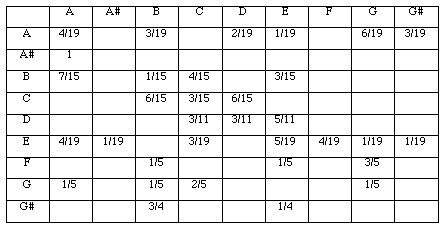
Figure 8 A Transition Table for a First-Order Markov Process
In general, as the order of the process increases, the sparsity of the matrix increases. Using this technique, a Nth order Markov Process requires an N+1 dimensioned transition table.
The transition table for a first-order Markov process description of Black Orpheus appears in Figure 8. It is possible to transform this transition table into a Markov diagram but the results are cluttered. The advantage of using the transition table is that it provides a compact and convenient form for representing and programming first-order stochastic processes. Using this technique, a Nth order Markov Process requires an N+1 dimensioned transition table.
Suppose we wish to compute Markov process probability tables from order 0 to 9 and store the results in the computer's memory (for the purpose of interactive composition we use the numeric keypad numbers 0 to 9). In general, the number of cells needed in all Nth order stochastic processes from 0..9 involving p pitch classes has
 (1.3-7)
elements when all the Nth order processes are stored in N+1-dimensioned matrices. Any attempt to reduce this number, f(12, 9) ~ 6.75x10^10, may be foiled by the introduction of pathologic data created by an advisary. For example, a large number of random numbers (much larger than the number of elements in the matrices) will eventually fill all the elements in the matrices. Never the less, it is practical, for low values of N, to perform the computation as described above. For example, the following code computes the 1st order Markov chain for Black Orpheus appears in Figure 9.
procedure compute_1st_order
begin
subtract the order number to keep the window from exceeding the number
of notes i.e., number_of_notes - order, note, the number_of_notes > order
with notes do
for each (note1 and note2) in (note_array[i] and note_array[i+1]) do
increment the number_of_2nd_order_event[note1,note2]
normalize the probs in the 1st order matrix
end
procedure play_first_order_stochastic_note;
begin
pick = random(0,1)
use the current row to perform a biased choice
play the choice and store the next element
end; {play_first_order_stochastic_note}
Figure 9. Code for Computation of 1st Order Stochastic Composition
Using this approach, we can implement a second order Markov process using the data structure shown in Figure 10.
second_order_markov_array_type = record
probability: array[1..11, 1..11, 1..11] of real;
used: array[1..11, 1..11] of boolean;
current_i, current_j: integer;
end;
Figure 10. Data Structure for a Second Order Markov Array
We would find (using 1.3-7) that a 9th order stochastic process over a 12 tone systems must make use of 6.75x10^10 elements. To make matters worse, using a matrix approach requires that we iterate over zero elements when computing the cumulative mass function. One objective (for the interactive realization of Markov processes on small computers) is to minimize the time it takes to compute a branch between nodes in the Markov chain.
Algorithms are available that implement sparse matrices with space proportional to the number of elements (Press et al.). These sparse-matrix approaches will reduce the amount of space needed, but cannot address the issue of execution time reduction. Since many visited states have zero probability (using the matrix approach) the time that the computer program takes to compute a branch cannot be predicted. We have found that this creates an uneven play back of the Markov chain during a real-time performance. This is a primary motivation for our approach which uses space which is linear in the number of Markovian states.
For the first-order stochastic process, shown above, the Petri-table appear in Figure 11.
The following program implements a second order Markov process using a petri-net. Transition probabilities are defined as the conditional probabilities between the states.
      Name             Place        Enabling Tokens     probability     Next Place
       A                 p1                Ta            0.21052632     p1
       A                 p1                Tb            0.15789474     p3
       A                 p1                Td            0.10526316     p4
       A                 p1                Te            0.05263158     p5
       A                 p1                Tg            0.31578947     p6
       A                 p1               Tg#            0.15789474     p7


       A#                p2                Ta                1          p1

       B                 p3                Ta            0.46666667     p2
       B                 p3                Tb            0.06666667     p3
       B          p3                Tc                0.26666667        p4
Figure 11 A Fragment of a First-Order Petri Net Table.
The zero elements of the Markov table are removed, reducing the time it takes to compute a branch. The number of rows is equal to the number of transitions.
In order to implement the Petri-table, and take full advantage of the fact that the number of elements in the table is linear in the number of transitions in the stochastic process, we need to write a program which can read Petri-tables directly. First we establish a Petri-table file format for a Markov-chain which appears as place, probability, next-place. The file format appears in Figure 12.
             1               0.21052632                   1
             1               0.15789474                   3
             1               0.10526316                   4
             1               0.05263158                   5
             1               0.31578947                   6
             1               0.15789474                   7
             2               1.0                          1
             3               0.46666667                   2
Figure
12. The File Format for the Stochastic Petri Table.The columns appear in the order of place, probability, next-place.
The data-structure used to store the Petri-net, with the next states and probability is shown in Figure 13.
type
{petri_markov data types}
petri_row_record = record
place: integer;
probability: real;
next_place: integer;
end; {petri_row_record}
row_array_type = array[1..35] of petri_row_record;
petri_type = record
row_array: row_array_type;
number_of_rows: integer;
current_place: integer;
end; {petri_array_type}
var
petri: petri_type;
The following pseudo code plays a row in the petri-table:
procedure play_petri_row (var petri: petri_type);
{play one row in the petri-table implementations of the first order Markov chain}
{these Markov chains of love, wont let me be, yeah!}
var
i: integer;
place_name: integer;
cmf: real;
prob_pick: real; {a number between 0 and 1}
while_loop_not_done: boolean;
begin
cmf = 0; {compute the cumulative probability mass function}
prob_pick = random(0,1)
while_loop_not_done := true;
with petri do
begin
i := current_place;
place_name := row_array[i].place;
with row_array[i] do
begin
while (place_name = place) and (cdf < prob_pick) do
begin
cmf := cmf + probability;
i := i + 1; {move to next row}
end; {while place_name}
make_tone(scale_array[i], tone_time);
current_place := next_place;
end; {with row_array[i]}
end; {with petri}
end; {play_petri_row}
Figure 13. Code to Define Stochastic Petric Table Data Type
Here, CMF stands for the cumulative probability mass function (computed by summing the probabilities of each of the transition arcs). To better understand the above program, recall the Petri-table file shown in Figure 12. To play one row, we first pick a pseudo-random number from 0 to 1, inclusive. We then transition from one row of the Petri table to the next until the cumulative mass function exceeds our probability pick, when this occurs, we take the transition to the next place.
In case the cumulative mass function does not sum to one (due to round-off error), we provide a compound conditional in the while loop, "(place_name = place) and (cmf < prob_pick)", this keeps us within the petri-table row.
The Petri table is a faster method for realizing Markov chains than the Markov table because of the elimination of the zero elements. It would be even faster to store the cumulative mass function, rather than the probability mass function. This saves a floating-point addition as the program iterates over each element in the Petri-table. The transition matrix requires 144 reals for a first-order Markov process. The Petri table needs only 66 integers and 33 reals. Assuming that an integer is 2 bytes long and that a real is 4 bytes, there are 144x4 bytes per real or 576 bytes used for the Markov transition table and 66x2+33x4 = 264 bytes for the Petri table. This saving grows as an exponential function of the order of the Markov process.
Suppose we use the Black Orpheus example to compute a 2nd-order Markov chain. In order to speed execution, and eliminate the sparse matrices, we use a Petri-net. A partial Petri net implementation of a Markov chain is shown in Figure 12.
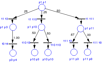
Figure 12 A Partial Stochastic Petri Net
The transition probabilities are shown on each arc. They indicate the probability of the occurrence of a token.
Here, we note that each of places has a transition probability that sums to one. Let R= row number of the Petri-table. N1, N2 and N3 = note 1 note 2 and note 3. Pijk is the probability that note k will occur given the occurrence of notes i and j. A partial Petri-table is shown in Figure 16.
R N1 N2 N3 Pijk
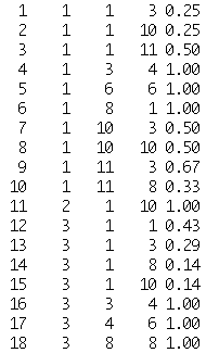
Figure 16. Partial Stochastic Petri Table
R is the row number of the table. N1 and N2 are two notes in the history of the Markov chain. N3 is the next note in the chain and Pijk is the probability that N3 will occur given the occurrence of notes N1 and N2.
In order to play such a table, a program must jump to a row given two notes. A procedure picks a uniformly distributed random number that varies from 0 to 1 (called r, this is created using linear congruential generator with a long period) (L'Ecuyer 1993). The procedure then sums the probabilities to form the cumulative mass function (CMF). When the CMF exceeds r, the value for the next state, k, is obtained.
In Petri-net parlance, k is a token that appears with a given probability. Note number two becomes the new note number one. K becomes the new note number two. An array (called the indirection array) gives us a pointer to the beginning of the list of places that start with note number 1.
An example indirection array is shown in Figure 17:
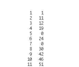
Figure 17 The Indirection Array.
The first element indicates the next note's pitch class. The second element points to the row in the Petri table the pitch class may be found. This keeps the procedure from having to perform a search for the next pitch class.
We have implemented 5th order stochastic processes using Petri nets. After that, the 100 note example tends to be deterministic.
In the future, we should eliminate the computation of the cumulative mass function by storing the cumulative mass function rather than the probability mass function. This should save the cost of an addition during the branching computation. In addition, we think that the computation of the stochastic Petri table may be made faster than the present implementation.
This author believes that the Markov chain method of computation may be of use in the area of animation and, in particular, dance. On this topic, as on many others relating to the use of stochastic Petri nets in the arts, much work remains to be done.
The source and Macintosh compiled version of the code for the program described in this article is available from the author for a 10$ fee to cover the cost of shipping and handling. It is also available through ftp to the site cse.bridgeport.edu.
Finally, I wish to acknowledge the debt I have to the late Mike Torello, who died while this paper was being written. Co-performer/Co-Composer and friend, Mike's influence and enthusiasm were infectious. He continues to be missed.
Apple. 1987. Apple Technical Introduction to the Macintosh Family. New York, New York: Addison-Wesley Publishing Company, Inc. , pp. 22, 169, 172.
Baggi, D. 1991. "Computer-Generated Music." Computer. 24(7):6-9.
Batish, S.D., and A. Batish. 1989. Ragopedia Volume 1. 1316 Mission St., Santa Cruz, California 96060: Batish Publications.
Dodge, C., and T. Jerse. 1985. Computer Music. New York, New York: Schimer Books.
Kassler. 1994. "Machine Models of Music." SIGART Bulletin. ACM Press, 5(1):51-52.
Katz, R. 1994. Contemporary Logic Design.. New York, New York: Benjamin/Cummings Publishing Company, Inc.
L'Ecuyer, P., F. Blouin, and R. Couture. 1993. "A Search for Good Multiple Recursive Random Number Generators." ACM Transactions on Modeling and Computer Simulation.. 3(2): 87-98.
Moore, F. R. 1990. Elements of Computer Music. Englewood Cliffs, New Jersey: Prentice Hall.
O'Haver, T. 1978. "More Music for the 6502." Byte. Peterborough, New Hampshire: Byte Publications, Inc., 3(6):140-141
Peterson, J. 1977. "Petri Nets." ACM Computing Surveys. 9(3):223-252.
Press, W., S. Teukolsky, W. Vetterling, and B. Flannery. 1992. Numerical Recipes in C. Cambridge, Massachusetts: Cambridge University Press.
Ralston, A. 1983. Encyclopedia of Computer Science and Engineering. Second Edition, , NY, NY: Van Nostrand Reinhold Company.
Randel, D. 1990. Harvard Concise Dictionary of Music. The Belknap Press of Cambridge, Massachusetts: Harvard University Press.
Roads, C., and J. Strawn, Eds. 1985. Foundations of Computer Music. Cambridge, Massachusetts: MIT Press.
Schwanauer, S., and D. Levitt. 1993. Machine Models of Music. Cambridge, Massachusetts: MIT Press.
Symantec Corporation. 1991.Think Pascal(TM) User Manual. Cupertino, California.
The International MIDI Association. 1990. Midi 1.0 Detailed Specification.. 5316 W. 57th St., Los Angles, California 90056, (213)649-6434: International MIDI Association.
Winsor, P. 1987. Computer-Assisted Music Composition.. Princeton, New Jersey: Petrocelli Books.